
データサイエンスとML(第48回):Transformerは取引において重要なのか

内容
- Transformerモデルとは
- 背景
- Transformerモデルアーキテクチャ
- TFT (Temporal Fusion Transformer)モデル
- TFTモデル用のデータ準備
- TFTの学習
- TFTモデルの最適パラメータ探索
- TFTモデルを自動売買ロボットに組み込む
- 結論
Transformerモデルとは
ディープラーニングにおいて、Transformerとはマルチヘッドアテンション機構に基づくニューラルネットワークアーキテクチャです。このアーキテクチャは、Googleの8名の研究者によって執筆された2017年の論文「Attention Is All You Need」で初めて提案されました。この論文では、Bahdanauらが2014年に提案したアテンション機構を発展させた新しいモデルが紹介され、現代AIの基盤技術の一つとして広く認識されています。
Transformerはさまざまな分野で顕著な成果を上げています。自然言語処理(NLP)の分野では、機械翻訳、感情分析、文章要約などで高い性能を示しています。また、画像処理分野にも応用され、画像分類や物体検出などのビジョンタスクでも成功を収めています。さらに、時系列分析への適用も進んでおり、長期依存関係を捉える能力により、株価予測や気象予測などのシーケンシャルデータの予測タスクでも有効性が示されています。
なお、本記事で使用する「Transformer」という用語は、単一の固定モデルではなく、アテンション機構を基盤とする一連のアーキテクチャ群を指します。
Transformerは、再帰構造ではなくアテンション機構を中心に構築されたニューラルネットワークアーキテクチャの総称です。従来の系列モデルとは異なり、系列内の各要素が他のすべての要素に直接注意(Attention)を向けることができるため、長距離依存関係のモデリングと並列計算による効率的な学習が可能になります。
もともとは自然言語処理向けに開発されましたが、その後、画像認識や時系列予測にも応用されるようになりました。特に時系列分野では、将来既知の入力、マルチホライズン予測(Multi-Horizon Forecasting)、データ量の制約といったドメイン固有の課題に対応するため、さまざまな派生アーキテクチャが提案されています。
背景
自然言語処理(NLP)の分野では、RNN (Recurrent Neural Network)やLSTM (Long Short-Term Memory)といった逐次モデルが広く利用されてきました。これらのモデルは機械翻訳や言語モデリングなどのタスクで優れた性能を示してきましたが、系列データを処理する際に構造上の制約を抱えています。
主な制約は以下の通りです。

従来の逐次モデルの構造
計算時間が長い
従来の逐次モデルでは、現在の時刻の情報を解釈するために、前の時刻までの情報を入力として利用します。図1の例にあるように、隠れ特徴量が段階的に処理される構造では、計算時間は入力長に対して線形にスケールします。そのため、系列が長くなるにつれて非効率性が増大します。
長距離依存関係の学習の難しさ
リカレントニューラルネットワーク(RNN)モデルはその逐次的な性質により、系列内の離れた要素間の依存関係を捉えることが困難です。LSTMやGRUといったアーキテクチャはこの問題を緩和するために導入されましたが、それでも固定サイズの隠れ状態表現に依存しているため、極めて長い系列を効果的に処理する能力には限界があります。
Googleの研究者たちは、再帰構造を完全に排除し、代わりにアテンション機構に基づいて入力および出力要素間のグローバルな依存関係を構築するTransformerモデルを提案しました。このアーキテクチャは、上述の制約を効果的に解決し、モデルのスケーラビリティと効率性を向上させることを目的としています。ただし、時系列など特定のドメインでは、近年の派生モデルにおいて再び再帰構造が導入される場合もあります。
Transformerモデルアーキテクチャ
![]()
自己注意機構(Self-Attention Mechanism)
従来のリカレントニューラルネットワーク(RNN)や長短期記憶(LSTM)ニューラルネットワークとは異なり、Transformerは自己注意機構に依存しており、入力系列内の異なる部分の重要度を重み付けしながら予測をおこなうことを可能にします。
並列化
Transformerは学習時の並列化を可能にしますが、一部の派生モデルでは推論時に逐次的処理が残る場合もあります。これにより、RNNのような逐次モデルと比較してより効率的な学習が可能となり、学習時間の短縮にもつながります。
エンコーダ・デコーダ構造
本モデルはエンコーダとデコーダから構成されます。エンコーダは入力系列を処理し文脈情報を抽出し、デコーダは出力系列を生成します。
マルチヘッドアテンション
自己注意機構は複数のヘッドへと拡張されており、入力系列の異なる側面に同時に注目することが可能になります。これにより、複雑な関係性をより適切に捉えることができます。
固定サイズの隠れ状態とは異なり、アテンション機構は系列内の任意の位置から関連情報を動的に選択することが可能です。
位置エンコーディング
Transformerは入力系列の順序を本質的には理解しません。そのため、トークンの位置情報を提供するために位置エンコーディングが入力埋め込みに加えられます。
なお、「Transformer」という用語は常に単一のモデルを指すわけではなく、アーキテクチャは用途によって大きく異なります。例は以下の通りです。
| モデル | アーキテクチャ | 主な用途/ドメイン |
|---|---|---|
| オリジナルTransformer | エンコーダ・デコーダ | 機械翻訳、sequence-to-sequence処理 |
| BERT (Bidirectional Encoder Representations from Transformers) | エンコーダのみ | テキスト理解(分類、NER、埋め込み) |
| GPT (Generative Pre-trained Transformer) | デコーダのみ | テキスト生成、言語モデリング、コード生成 |
| ViT (Vision Transformer) | エンコーダのみ | 画像分類、視覚表現学習 |
| TFT (Temporal Fusion Transformer) | ハイブリッド(LSTM + アテンション) | 時系列予測、財務データ、ビジネスデータ |
Transformerがどのように構成されているかに関する詳細情報やその他の内容については、本記事の末尾にある参考文献セクションをご参照ください。
数あるTransformerモデルの中でも、TFTは時系列予測に適したモデルです。本記事では、TFTの概要を説明した後、その実装方法と市場予測への応用について解説します。
TFT (Temporal Fusion Transformer)モデル
TFTは次のように定義されています。
TFTは、マルチホライズン時系列予測のために設計された、最先端のアテンションベースの深層学習モデルです。
このモデルはGoogleとオックスフォード大学の研究者らによって提案されたもので、記事中では2021年のものとして扱っています。LSTM (Long Short-Term Memory)ベースのエンコーダ・デコーダ構造と自己注意機構を組み合わせることで、高性能かつ解釈可能な予測を実現するよう設計されています。
TFTの理論およびアーキテクチャの詳細については、https://medium.com/dataness-ai/understanding-temporal-fusion-transformer-9a7a4fcde74bをご覧ください。
PyTorch-forecastingフレームワークを使用してこのモデルを実装しましょう。
まず、このプロジェクトで使用するすべての依存関係(本記事末尾に添付されているzipファイル内のrequirements.txtファイルに含まれています)をPython仮想環境にインストールします。
pip install -r requirements.txt
TFTモデル用のデータ準備
まず、MetaTrader 5ターミナルからデータをインポートします。
import MetaTrader5 as mt5

# Get rates from the MetaTrader5 app

if not mt5.initialize():
    print("initialize() failed, error code =", mt5.last_error())
    quit()

symbol = "EURUSD"
rates = mt5.copy_rates_from_pos(symbol, mt5.TIMEFRAME_M15, 0, 10000)
rates_df = pd.DataFrame(rates)

rates_df["time"] = pd.to_datetime(rates_df["time"], unit="s")
data = pd.concat([rates_df, get_features(rates_df)], axis=1)
特徴量エンジニアリング
受け取った特徴量すべてを使う必要はありません。不要と思われる特徴量は削除します。
rates_df.drop(columns=[
            "spread",
            "real_volume"
        ], inplace=True)
この操作後の残りの特徴量も十分ではないので、DataFrameに新しい特徴量を追加します。
以下は、さまざまな特徴量(特徴量エンジニアリングによる新しい変数)を導入するのに役立つシンプルなクラスです。
features.py
- 日付と時刻に基づく特徴量
features.py
import pandas as pd
from ta.trend import sma_indicator, ema_indicator, macd_diff, macd_signal
from ta.momentum import stochrsi_k, stochrsi_d, rsi
from ta.volatility import bollinger_hband, bollinger_lband

class FeatureEngineer:

    # date/time features

    @staticmethod
    def hour(date_series: pd.Series) -> pd.Series:
        return date_series.dt.hour

    @staticmethod
    def dayofweek(date_series: pd.Series) -> pd.Series:
        return date_series.dt.dayofweek

    @staticmethod
    def dayofmonth(date_series: pd.Series) -> pd.Series:
        return date_series.dt.day

    @staticmethod
    def month(date_series: pd.Series) -> pd.Series:
        return date_series.dt.month
- トレンドフォロー指標
    # trend following indicators

    @staticmethod
    def sma(price: pd.Series, window: int=20) -> pd.Series:
        return sma_indicator(price, window)

    @staticmethod
    def ema(price: pd.Series, window: int=20) -> pd.Series:
        return ema_indicator(price, window)

    @staticmethod
    def macd_diff(price: pd.Series, window_slow: int=26, window_fast: int=12, window_signal: int=9) -> pd.Series:
        return macd_diff(price, window_slow=window_slow, window_fast=window_fast, window_sign=window_signal)

    @staticmethod
    def macd_signal(price: pd.Series, window_slow: int=26, window_fast: int=12, window_signal: int=9) -> pd.Series:
        return macd_signal(price, window_slow=window_slow, window_fast=window_fast, window_sign=window_signal
- モメンタム指標
    # momentum indicators

    @staticmethod
    def rsi(price: pd.Series, window: int=14) -> pd.Series:
        return rsi(price, window)

    @staticmethod
    def stochrsi_k(price: pd.Series, window: int=14, smooth1: int=3, smooth2: int=3) -> pd.Series:
        return stochrsi_k(price, window=window, smooth1=smooth1, smooth2=smooth2)

    @staticmethod
    def stochrsi_d(price: pd.Series, window: int=14, smooth1: int=3, smooth2: int=3) -> pd.Series:
        return stochrsi_d(price, window=window, smooth1=smooth1, smooth2=
- ボラティリティ指標
    # volatility indicators

    @staticmethod
    def bollinger_hband(price: pd.Series, window: int=20, window_dev: int=2) -> pd.Series:
        return bollinger_hband(price, window=window, window_dev=window_dev)

    @staticmethod
    def bollinger_lband(price: pd.Series, window: int=20, window_dev: int=2) -> pd.Series:
        return bollinger_lband(price, window=window, window_dev=window_dev)
このクラスのメソッドは、同じクラス内のget_allという単一の静的関数内で呼び出されます。
    @staticmethod
    def get_all(data: pd.DataFrame) -> pd.DataFrame:

        return pd.DataFrame({
            "hour": FeatureEngineer.hour(data["time"]),
            "dayofweek": FeatureEngineer.dayofweek(data["time"]),
            "dayofmonth": FeatureEngineer.dayofmonth(data["time"]),
            "month": FeatureEngineer.month(data["time"]),
            "sma_20": FeatureEngineer.sma(data["close"]),
            "ema_20": FeatureEngineer.ema(data["close"]),
            "macd_diff": FeatureEngineer.macd_diff(data["close"]),
            "macd_signal": FeatureEngineer.macd_signal(data["close"]),
            "rsi": FeatureEngineer.rsi(data["close"]),
            "stochrsi_k": FeatureEngineer.stochrsi_k(data["close"]),
            "stochrsi_d": FeatureEngineer.stochrsi_d(data["close"]),
            "bollinger_hband": FeatureEngineer.bollinger_hband(data["close"]),
            "bollinger_lband": FeatureEngineer.bollinger_lband(data["close"]),
        })
このクラスを使用して、特徴量で構成された新しいPandas-DataFrameを取得します。
new_features = features.FeatureEngineer.get_all(rates_df)
以下が実行結果です。
(.env) C:\Users\Omega Joctan\OneDrive\mql5 articles\Data Science and ML\Part 48\TFT>python train.py
      hour  dayofweek  dayofmonth  month    sma_20    ema_20  macd_diff  macd_signal        rsi  stochrsi_k  stochrsi_d  bollinger_hband  bollinger_lband
0       20          3          21      8       NaN       NaN        NaN          NaN        NaN         NaN         NaN              NaN              NaN
1       20          3          21      8       NaN       NaN        NaN          NaN        NaN         NaN         NaN              NaN              NaN
2       20          3          21      8       NaN       NaN        NaN          NaN        NaN         NaN         NaN              NaN              NaN
3       20          3          21      8       NaN       NaN        NaN          NaN        NaN         NaN         NaN              NaN              NaN
4       21          3          21      8       NaN       NaN        NaN          NaN        NaN         NaN         NaN              NaN              NaN
...    ...        ...         ...    ...       ...       ...        ...          ...        ...         ...         ...              ...              ...
9985    20          4          16      1  1.160491  1.160265  -0.000107    -0.000404  41.591063    0.303937    0.316652         1.162598         1.158383
9986    20          4          16      1  1.160384  1.160213  -0.000068    -0.000421  43.685146    0.499779    0.367431         1.162418         1.158349
9987    20          4          16      1  1.160269  1.160151  -0.000047    -0.000433  42.436779    0.698607    0.500775         1.162214         1.158323
9988    21          4          16      1  1.160154  1.160067  -0.000046    -0.000444  40.194753    0.774743    0.657710         1.162051         1.158257
9989    21          4          16      1  1.160052  1.160010  -0.000026    -0.000450  42.452830    0.687333    0.720228         1.161864         1.158240

[9990 rows x 13 columns]
その後、両方のDataFrameを結合し、最終的なモデル学習に使用するより大きなDataFrameを作成します。
data = pd.concat([rates_df, new_features], axis=1) # concatenate dataframes
以下が実行結果です。
                    time     open     high      low    close  tick_volume  ...  macd_signal        rsi  stochrsi_k  stochrsi_d  bollinger_hband  bollinger_lband
0    2025-08-21 20:00:00  1.16112  1.16171  1.16112  1.16170          642  ...          NaN        NaN         NaN         NaN              NaN              NaN
1    2025-08-21 20:15:00  1.16170  1.16173  1.16126  1.16136          557  ...          NaN        NaN         NaN         NaN              NaN              NaN
2    2025-08-21 20:30:00  1.16136  1.16167  1.16129  1.16158          414  ...          NaN        NaN         NaN         NaN              NaN              NaN
3    2025-08-21 20:45:00  1.16158  1.16187  1.16149  1.16151          513  ...          NaN        NaN         NaN         NaN              NaN              NaN
4    2025-08-21 21:00:00  1.16151  1.16152  1.16103  1.16106          473  ...          NaN        NaN         NaN         NaN              NaN              NaN
...                  ...      ...      ...      ...      ...          ...  ...          ...        ...         ...         ...              ...              ...
9985 2026-01-16 20:15:00  1.15911  1.15954  1.15905  1.15951          407  ...    -0.000404  41.591063    0.303937    0.316652         1.162598         1.158383
9986 2026-01-16 20:30:00  1.15951  1.15973  1.15936  1.15972          289  ...    -0.000421  43.685146    0.499779    0.367431         1.162418         1.158349
9987 2026-01-16 20:45:00  1.15972  1.15994  1.15955  1.15956          447  ...    -0.000433  42.436779    0.698607    0.500775         1.162214         1.158323
9988 2026-01-16 21:00:00  1.15956  1.15967  1.15921  1.15927          457  ...    -0.000444  40.194753    0.774743    0.657710         1.162051         1.158257
9989 2026-01-16 21:15:00  1.15927  1.15958  1.15915  1.15947          290  ...    -0.000450  42.452830    0.687333    0.720228         1.161864         1.158240

[9990 rows x 19 columns]
目的変数の作成
典型的な教師あり機械学習では、モデルが他の特徴量(説明変数)を用いて予測すべき目的変数が必要になります。
今回のような時系列問題では、リターンをターゲット変数として使用します。
data["returns"] = data["close"].pct_change()
時系列データセットオブジェクトの作成
PyTorch-forecastingでは、モデル用のデータを、TimeSeriesDatasetと呼ばれるオブジェクトに格納する必要があります。
そのためには、TimeSeriesDatasetに渡す前に、DataFrame内にtime_idxという列を用意する必要があります。
data["time_idx"] = data.index
data.drop(columns=["time"], inplace=True)
これは、データ内の時間インデックスを表す整数型の列です。この列はサンプルの系列を決定するために使用されます。観測値に欠損がない場合、時間インデックスは各サンプルごとに+1ずつ増加する必要があります。各系列の最初のtime_idxは必ずしも0である必要はなく、任意の値を取ることができます。
time_idx列をDataFrameに追加した後は、元の時間(datetime)を含む列は削除する必要があります(TFTはdatetime変数を直接使用しないためです)。
data.drop(columns=["time"], inplace=True)
max_prediction_length = 6
max_encoder_length = 24
training_cutoff = data["time_idx"].max() - max_prediction_length

training = TimeSeriesDataSet(
    data[lambda x: x.time_idx <= training_cutoff],
    time_idx="time_idx",
    target="returns",
    group_ids=["symbol"],
    min_encoder_length=max_encoder_length // 2,  # keep encoder length long (as it is in the validation set)
    max_encoder_length=max_encoder_length,
    min_prediction_length=1,
    max_prediction_length=max_prediction_length,
    static_categoricals=["symbol"],
    # time_varying_known_categoricals=[],

    time_varying_known_reals=[
                            "hour",
                            "dayofweek",
                            "dayofmonth",
                            "month",
                            "time_idx",
                            "stochrsi_k",
                            "stochrsi_d",
                            "rsi",
                            "macd_diff",
                            ],

    time_varying_unknown_categoricals=[],
    time_varying_unknown_reals=[
        "open",
        "high",
        "low",
        "close",
        "tick_volume",
        "ema_20",
        "sma_20",
        "bollinger_hband",
        "bollinger_lband"
    ],

    target_normalizer=GroupNormalizer(
        groups=["symbol"], transformation="softplus"
    ),  # use softplus and normalize by group

    add_target_scales=True,
    add_encoder_length=True,
)
このオブジェクトは多くの変数を受け取ります。以下の表はそれらのいくつかを示しています。(詳細はこちら)。
| 変数 | 詳細 |
|---|---|
| max_encoder_length | モデルが参照できる過去の期間 |
| max_prediction_length | モデルが予測しなければならない未来の期間 |
| time_varying_known_reals | 時間とともに変化し、かつ将来の値が既知である連続変数のリスト 今回のケースでは、DataFrameに含まれる定常指標および時間特徴量を選択しています。 |
| time_varying_unknown_reals | 将来の値が未知であり、時間とともに変化する連続変数のリスト。実際の目的変数もここに含めます。 このため、open、high、low、closeなどの特徴量を選択しています。これらは将来の値が不確実な特徴量です。 |
| group_ids | データ内の時系列インスタンスを識別するための列名リスト。group_idsはtime_idxと組み合わせて1つのサンプルを定義します。単一の時系列しかない場合は、一定の値を持つ列名を指定します。 Pandas DataFrameにはシンボルが1つしか収集されていないため、割り当てるグループは現在のシンボルのみとなります。 data["symbol"] = "EURUSD"グループは、異なる通貨ペア(銘柄)や時間足など、複数の時系列データを表すこともあります。 |
最後に、学習用オブジェクトを模倣して検証データを作成します。
#  (predict=True) which means to predict the last max_prediction_length points in time for each series

validation = TimeSeriesDataSet.from_dataset(
    training, data, predict=True, stop_randomization=True
)
最後に、学習データと検証データの両方に対して、 PyTorchデータローダーを作成します(データローダーは、モデルにデータを供給するのに適しています)。
batch_size = 128  # set this between 32 to 128
train_dataloader = training.to_dataloader(
    train=True, batch_size=batch_size, num_workers=0
)
val_dataloader = validation.to_dataloader(
    train=False, batch_size=batch_size * 10, num_workers=0
)
TFTの学習
PyTorch Lightningを使用してモデルをトレーニングします。以下はトレーニングタスク用のLightningトレーナーです。
pl.seed_everything(42) # random seed for reproducibility

lr_logger = LearningRateMonitor()  # log the learning rate
logger = TensorBoardLogger("lightning_logs")  # logging results to a tensorboard

# configure network and trainer
early_stop_callback = EarlyStopping(
    monitor="val_loss", min_delta=1e-4, patience=10, verbose=False, mode="min"
)

trainer = pl.Trainer(
    max_epochs=50,
    accelerator="cpu",
    enable_model_summary=True,
    gradient_clip_val=0.1,
    limit_train_batches=50,  # comment in for training, running validation every 30 batches
    # fast_dev_run=True,  # comment in to check that networkor dataset has no serious bugs
    callbacks=[lr_logger, early_stop_callback],
    logger=logger,
)
モデルにとって最適な学習率を事前に知る方法はないため、適切な学習率を探索することにします。
まず、最適な学習率を見つけるために使用するTFTモデルのインスタンスを作成します。
tft = TemporalFusionTransformer.from_dataset(
    training,
    # not meaningful for finding the learning rate but otherwise very important
    learning_rate=0.03,
    hidden_size=8,  # most important hyperparameter apart from learning rate
    # number of attention heads. Set to up to 4 for large datasets
    attention_head_size=2,
    dropout=0.1,  # between 0.1 and 0.3 are good values
    hidden_continuous_size=8,  # set to <= hidden_size
    loss=metrics.QuantileLoss(),
    optimizer="ranger",
    # reduce learning rate if no improvement in validation loss after x epochs
    # reduce_on_plateau_patience=1000,
)
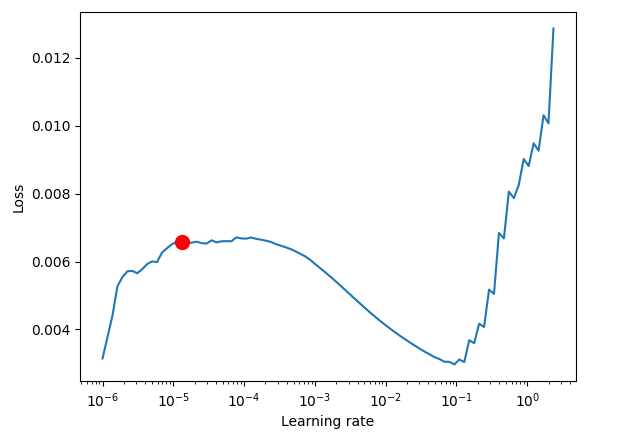
最適な学習率を見つけます。
res = Tuner(trainer).lr_find(
    tft,
    train_dataloaders=train_dataloader,
    val_dataloaders=val_dataloader,
    max_lr=10.0,
    min_lr=1e-6,
)

optimal_lr = res.suggestion()

print(f"suggested learning rate: {optimal_lr}")
fig = res.plot(show=False, suggest=True)

plots_path = os.path.join(outputs_dir, "Plots")
os.makedirs(plots_path, exist_ok=True)

fig.savefig(os.path.join(plots_path, "lr_finder.png"))
以下が実行結果です。
Finding best initial lr:  91%|█████████████████████████████████████████████████████████████████████████████████████████████▋         | 91/100 [00:41<00:04,  2.20it/s]
LR finder stopped early after 91 steps due to diverging loss.
Restoring states from the checkpoint path at C:\Users\Omega Joctan\OneDrive\mql5 articles\Data Science and ML\Part 48\TFT\.lr_find_6df0be87-4347-4325-98f1-3a2b5a244c46.ckpt
Restored all states from the checkpoint at C:\Users\Omega Joctan\OneDrive\mql5 articles\Data Science and ML\Part 48\TFT\.lr_find_6df0be87-4347-4325-98f1-3a2b5a244c46.ckpt
Learning rate set to 1.3182567385564071e-05
suggested learning rate: 1.3182567385564071e-05
最適な学習率が得られたら、新しいモデルインスタンスを作成し、その学習率の値を用いて学習させます。
tft = TemporalFusionTransformer.from_dataset(
    training,
    learning_rate=optimal_lr,
    hidden_size=16,
    attention_head_size=2,
    dropout=0.1,
    hidden_continuous_size=8,
    loss=metrics.QuantileLoss(),
    log_interval=10,  # uncomment for learning rate finder and otherwise, e.g., to 10 for logging every 10 batches
    optimizer="ranger",
    reduce_on_plateau_patience=4,
)

print(f"Number of parameters in network: {tft.size() / 1e3:.1f}k")

trainer.fit(
    tft,
    train_dataloaders=train_dataloader,
    val_dataloaders=val_dataloader,
)

tft_predictions = tft.predict(val_dataloader, return_y=True)
print("TFT MAE: ", metrics.MAE()(tft_predictions.output, tft_predictions.y))
以下が実行結果です。
Epoch 4: 100%|██████████████████████████████████████████| 50/50 [01:04<00:00,  0.77it/s, v_num=1, train_loss_step=0.000846, val_loss=0.0013, train_loss_epoch=0.00092]`Trainer.fit` stopped: `max_epochs=5` reached.
Epoch 4: 100%|██████████████████████████████████████████| 50/50 [01:05<00:00,  0.77it/s, v_num=1, train_loss_step=0.000846, val_loss=0.0013, train_loss_epoch=0.00092]
💡 Tip: For seamless cloud uploads and versioning, try installing [litmodels](https://pypi.org/project/litmodels/) to enable LitModelCheckpoint, which syncs automatically with the Lightning model registry.
GPU available: False, used: False
TPU available: False, using: 0 TPU cores
TFT MAPE:  tensor(1.2644)+
モデルによる予測値と実際の値を比較して可視化することで、モデルの予測値が真の値(元の値)と比べてどの程度の精度なのかを把握してみましょう。
best_model_path = trainer.checkpoint_callback.best_model_path
best_tft = TemporalFusionTransformer.load_from_checkpoint(best_model_path)

# raw predictions are a dictionary from which all kinds of information, including quantiles, can be extracted
raw_predictions = best_tft.predict(
    val_dataloader, mode="raw", return_x=True, trainer_kwargs=dict(accelerator="cpu")
)

n = raw_predictions.output.prediction.shape[0]
print(f"Plotting {n} predictions...")

for idx in range(n):
    fig = best_tft.plot_prediction(
        raw_predictions.x,
        raw_predictions.output,
        idx=idx,
        add_loss_to_title=True
    )

    fig.savefig(os.path.join(plots_path, f"tft_prediction_{idx}.png"))
    plt.close(fig=fig)
以下が実行結果です。
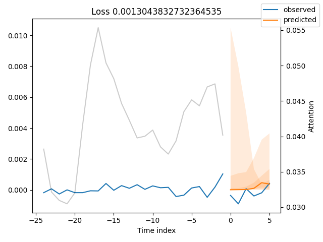
予測値は元の値にかなり近い結果となっているようです。
ただし、MAE(平均絶対誤差)という指標は単体では意味を持たず、比較対象があって初めて評価できます。そのため、他のモデルと比較する必要があります。そこで、ベースラインモデルを用いて確認します。
ベースラインモデル
ベースラインモデルとは、直前の既知のターゲット値をそのまま予測値として使用するシンプルなモデルです。これは、モデルが最低限上回るべき基準となる指標を提供します。
baseline_predictions = Baseline().predict(val_dataloader, return_y=True)
print("Baseline model MAE: ",metrics.MAE()(baseline_predictions.output, baseline_predictions.y))
上記のスクリプトを再度実行した結果、TFTモデルはベースラインモデルの約2倍の精度を達成しました。
TFT MAE:  tensor(0.0002)
Baseline model MAE:  tensor(0.0004)
TFTモデルの最適パラメータ探索
Transformerベースのモデルはニューラルネットワークの一種であり(内部にLSTMも含まれています)、他のニューラルネットワークと同様にハイパーパラメータに強く依存します。
そのため、問題に応じて最適なハイパーパラメータを見つけることが重要です。
ドキュメントによると、
PyTorch Forecastingではoptunaを用いたハイパーパラメータチューニングが標準でサポートされており、optimize_hyperparameters 関数を使ってTFTの最適化をおこなうことができます。
例は以下の通りです。
import pickle

from pytorch_forecasting.models.temporal_fusion_transformer.tuning import optimize_hyperparameters

# create study
study = optimize_hyperparameters(
    train_dataloader,
    val_dataloader,
    model_path="optuna_test",
    n_trials=200,
    max_epochs=50,
    gradient_clip_val_range=(0.01, 1.0),
    hidden_size_range=(8, 128),
    hidden_continuous_size_range=(8, 128),
    attention_head_size_range=(1, 4),
    learning_rate_range=(0.001, 0.1),
    dropout_range=(0.1, 0.3),
    trainer_kwargs=dict(limit_train_batches=30),
    reduce_on_plateau_patience=4,
    use_learning_rate_finder=False,  # use Optuna to find ideal learning rate or use in-built learning rate finder
)

# save study results - also we can resume tuning at a later point in time
with open("test_study.pkl", "wb") as fout:
    pickle.dump(study, fout)

# show best hyperparameters
print(study.best_trial.params)
scikit-learnやKerasといった他の機械学習用Pythonフレームワークとは異なり、PyTorchのモジュールではある程度手動でコードを書く必要があり、その結果として多くの処理を個別に実装しなければならないことがよくあります。これは、コーディング作業を煩雑にしたり、バグの原因になったりすることがあります。
そこで、作業をより簡単にするために、必要なコードをすべて一つのクラスにまとめてラップすることにします。
model.py
class TFTModel:
    def __init__(self, training: TimeSeriesDataSet,
                train_dataloader: DataLoader,
                val_dataloader: DataLoader,
                parameters: dict,
                loss: metrics=metrics.QuantileLoss(),
                trainer_max_epochs = 10):

        """
        Initialize the Temporal Fusion Transformer model with training and validation data.
        Args:
            training (TimeSeriesDataSet): The training dataset loader containing time series data
                for model training.
            parameters (dict): A dictionary containing hyperparameters for the model configuration:
                - learning_rate (float, optional): Learning rate for the optimizer. Default is 0.03.
                - hidden_size (int, optional): Size of hidden layers. Most important hyperparameter apart
                  from learning rate. Default is 8.
                - attention_head_size (int, optional): Number of attention heads. Set to up to 4 for
                  large datasets. Default is 2.
                - dropout (float, optional): Dropout rate for regularization. Values between 0.1 and 0.3
                  are recommended. Default is 0.1.
                - hidden_continuous_size (int, optional): Size of continuous hidden layers. Should be set
                  to <= hidden_size. Default is 8.
            loss (metrics): Loss function to be used for model training, e.g., QuantileLoss.
        Attributes:
            model (TemporalFusionTransformer): The initialized Temporal Fusion Transformer model with
                a given loss function and Ranger optimizer.
            trainer: PyTorch Lightning trainer instance configured for model training.
        """

        # configure network and trainer
        pl.seed_everything(42)

        self.train_dataloader = train_dataloader
        self.val_dataloader = val_dataloader
        self.training = training
        self.loss = loss

        self.model = self._create_model(parameters=parameters)
        self.trainer = self._create_trainer(max_epochs=trainer_max_epochs)

    def _create_model(self, parameters: dict) -> TemporalFusionTransformer:

        return TemporalFusionTransformer.from_dataset(
            self.training,
            # not meaningful for finding the learning rate but otherwise very important
            learning_rate=parameters.get("learning_rate", 0.03),
            hidden_size=parameters.get("hidden_size", 8),  # most important hyperparameter apart from learning rate
            # number of attention heads. Set to up to 4 for large datasets
            attention_head_size=parameters.get("attention_head_size", 2),
            dropout=parameters.get("dropout", 0.1),  # between 0.1 and 0.3 are good values
            hidden_continuous_size=parameters.get("hidden_continuous_size", 8),  # set to <= hidden_size
            loss=self.loss,
            optimizer="ranger",
            # reduce learning rate if no improvement in validation loss after x epochs
            # reduce_on_plateau_patience=1000,
        )

    def _create_trainer(self, max_epochs: int=50, grad_clip_val=0.1, limit_train_batches: int=50) -> pl.Trainer:

        lr_logger = LearningRateMonitor()  # log the learning rate
        logger = TensorBoardLogger("lightning_logs")  # logging results to a tensorboard

        # configure network and trainer
        early_stop_callback = EarlyStopping(
            monitor="val_loss", min_delta=1e-4, patience=10, verbose=False, mode="min"
        )

        return pl.Trainer(
            max_epochs=max_epochs,
            accelerator="cpu",
            enable_model_summary=True,
            gradient_clip_val=grad_clip_val,
            limit_train_batches=limit_train_batches,  # comment in for training, running validation every 30 batches
            # fast_dev_run=True,  # comment in to check that networkor dataset has no serious bugs
            callbacks=[lr_logger, early_stop_callback],
            logger=logger,
        )


    def find_optimal_lr(self, plot_output_dir: str,
                        max_lr: float=10.0,
                        min_lr: float=1e-6,
                        show_plot: bool=False,
                        save_plot: bool=True) -> float:

        """find an optimal learning rate"""

        res = Tuner(self.trainer).lr_find(
            self.model,
            train_dataloaders=self.train_dataloader,
            val_dataloaders=self.val_dataloader,
            max_lr=max_lr,
            min_lr=min_lr,
        )

        optimal_lr = res.suggestion()

        # ---- optional, saving the plot ----

        fig = res.plot(show=show_plot, suggest=True)

        if save_plot:
            try:
                fig.savefig(os.path.join(plot_output_dir, "lr_finder.png"))
            except Exception as e:
                print("Error saving learning rate finder plot: ", e)

        return optimal_lr

    def load_best_model(self) -> bool:

        """Load the best model checkpoint after training."""

        model = None

        try:
            best_model_path = self.trainer.checkpoint_callback.best_model_path
            model = TemporalFusionTransformer.load_from_checkpoint(best_model_path)
        except Exception as e:
            print("Error loading best model checkpoint: ", e)
            return False

        self.model = model
        return True

    def fit(self):
        self.trainer.fit(
            self.model,
            train_dataloaders=self.train_dataloader,
            val_dataloaders=self.val_dataloader,
        )

    def predict(self, x: TimeSeriesDataSet,  return_x: Optional[bool]=False, mode: Optional[str]="prediction", return_y: bool=True):

        try:
            tft_predictions = self.model.predict(x, mode=mode, return_x=return_x, return_y=return_y)
        except Exception as e:
            print(f"Failed to predict: {e}")
            return None

        return tft_predictions

    @staticmethod
    def find_optimal_parameters(train_dataloader: TimeSeriesDataSet,
                                val_dataloader: TimeSeriesDataSet,
                                max_epochs: int=50,
                                n_trials: int=100,
                                use_learning_rate_finder: bool=False,
                                model_path: str="optuna_test",
                                best_params_path: str="best_params.pkl",
                                timeout: int=300) -> dict:

        """
        Find optimal hyperparameters for a Temporal Fusion Transformer model using Optuna. Best parameters are saved for potential later usage
        Args:
            train_dataloader (TimeSeriesDataSet): Training dataset loader containing time series data.
            val_dataloader (TimeSeriesDataSet): Validation dataset loader for evaluating model performance.
            max_epochs (int, optional): Maximum number of training epochs per trial. Defaults to 50.
            n_trials (int, optional): Number of optimization trials to run. Defaults to 100.
            use_learning_rate_finder (bool, optional): Whether to use built-in learning rate finder
                instead of Optuna-based learning rate optimization. Defaults to False.
            model_path (str, optional): Directory path to save model checkpoints during optimization.
                Defaults to "optuna_test".
            best_params_path (str, optional): File path to save the best hyperparameters.
                Defaults to "best_params.pkl".
            timeout (int, optional): Maximum time in seconds to run the optimization study.
                Defaults to 300.
        Returns:
            dict: Dictionary containing the best hyperparameters found during optimization.
        """

        # create study
        study = optimize_hyperparameters(
            train_dataloader,
            val_dataloader,
            model_path=model_path,
            n_trials=n_trials,
            max_epochs=max_epochs,
            gradient_clip_val_range=(0.01, 1.0),
            hidden_size_range=(8, 128),
            hidden_continuous_size_range=(8, 128),
            attention_head_size_range=(1, 4),
            learning_rate_range=(0.001, 0.1),
            dropout_range=(0.1, 0.3),
            trainer_kwargs=dict(limit_train_batches=30),
            reduce_on_plateau_patience=4,
            use_learning_rate_finder=use_learning_rate_finder,  # use Optuna to find ideal learning rate or use in-built learning rate finder
            timeout=timeout,  # stop study after given seconds
        )

        # save study results - also we can resume tuning at a later point in time

        best_params = study.best_trial.params
        try:
            with open(best_params_path, "wb") as fout:
                pickle.dump(best_params, fout)
                print("Best parameters saved to: ", best_params_path)
        except Exception as e:
            print("Error saving best parameters: ", e)

        # return best hyperparameters
        return best_params

    def plot_raw_predictions(self, raw_predictions, plots_path: str, show=False):

        n = raw_predictions.output.prediction.shape[0]
        print(f"Plotting {n} predictions...")

        for idx in range(n):
            fig = self.model.plot_prediction(
                raw_predictions.x,
                raw_predictions.output,
                idx=idx,
                add_loss_to_title=True
            )

            if show:
                plt.show(fig=fig)

            fig.savefig(os.path.join(plots_path, f"tft_prediction_{idx}.png"))
            plt.close(fig=fig)
クラスを用いることで、再利用可能なトレーナーの管理、モデルの学習、最適パラメータの探索などをより整理された形で扱うことができます。
たとえば、TFTModelクラス内にfind_optimal_parametersをstaticメソッドとして定義することで、クラスのインスタンスを生成する前にこの関数を実行し、最適なパラメータを取得することが可能になります。その後、その結果をクラスインスタンスに再度反映させることができます。
例は以下の通りです。
best_params = model.TFTModel.find_optimal_parameters(train_dataloader=train_dataloader,
                                            val_dataloader=val_dataloader,
                                            timeout=optuna_timeout,
                                            best_params_path=best_params_path
                                            )

    print("Best hyperparameters found: ", best_params)

    tft_model = model.TFTModel(
        training=training,
        train_dataloader=train_dataloader,
        val_dataloader=val_dataloader,
        parameters=best_params,
        trainer_max_epochs=max_training_epochs
    )
TFTモデルを自動売買ロボットに組み込む
実用的な自動売買ロボットを構築するためには、推論時においても市場の最新データを用いてモデルの予測値を取得する必要があります。
TFTでは、推論時にも学習時と同じ特徴量セット(目的変数を含む)が必要になるため、データ収集と特徴量エンジニアリングを一貫しておこなうためのグローバル関数を用意する必要があります。
bot.py
def prepare_data(rates_df: pd.DataFrame) -> pd.DataFrame:

    rates_df["time"] = pd.to_datetime(rates_df["time"], unit="s") # convert time in seconds to datetime

    features_df = features.FeatureEngineer.get_all(rates_df)
    data = pd.concat([rates_df, features_df], axis=1) # concatenate dataframes

    # making the target variable

    data["returns"] = data["close"].pct_change()
    data["symbol"] = "EURUSD" # assigning symbol name as a group

    # drop NANs if any

    data.dropna(inplace=True)

    # assigning a time index

    data = data.reset_index(drop=True)
    data["time_idx"] = data.index

    # let's keep track of unused features

    unused_features = ["time", "spread", "real_volume"]
    return data.drop(columns=unused_features)
上記の関数は、MetaTrader 5から取得した生のDataFrameを入力として受け取り、新しい特徴量を生成し、目的変数、グループ情報、時間インデックスなどを含む必要なすべての特徴量を整形したうえで、最終的にモデル学習に必要なデータセットを返します。
また、モデルをトレーニングするための関数も必要です。この関数は、学習済みのTFTModelインスタンスをグローバル変数として保持する役割を持つように設計します。
bot.py
def train_model(start_bar: int=100,
                num_bars: int=1000,
                symbol: int = "EURUSD",
                timeframe: int=mt5.TIMEFRAME_M15,
                max_prediction_length: int = 6,
                max_encoder_length: int = 24,
                load_best_parameters = False):

    # we extract training data from MetaTrader 5

    try:
        rates = mt5.copy_rates_from_pos(symbol, timeframe, start_bar, num_bars)
    except Exception as e:
        print("Error retrieving data from MetaTrader 5: ", e)
        return

    data = prepare_data(rates_df=pd.DataFrame(rates))

    # ------------ preparing training data and data loaders ------------

    training_cutoff = data["time_idx"].max() - max_prediction_length

    training = TimeSeriesDataSet(
        data[lambda x: x.time_idx <= training_cutoff],
        time_idx="time_idx",
        target="returns",
        group_ids=["symbol"],
        min_encoder_length=max_encoder_length // 2,  # keep encoder length long (as it is in the validation set)
        max_encoder_length=max_encoder_length,
        min_prediction_length=1,
        max_prediction_length=max_prediction_length,
        static_categoricals=["symbol"],
        # time_varying_known_categoricals=[],

        time_varying_known_reals=[
                                "hour",
                                "dayofweek",
                                "dayofmonth",
                                "month",
                                "time_idx",
                                "stochrsi_k",
                                "stochrsi_d",
                                "rsi",
                                "macd_diff",
                                ],

        time_varying_unknown_categoricals=[],
        time_varying_unknown_reals=[
            "open",
            "high",
            "low",
            "close",
            "tick_volume",
            "ema_20",
            "sma_20",
            "bollinger_hband",
            "bollinger_lband"
        ],

        target_normalizer=GroupNormalizer(
            groups=["symbol"], transformation="softplus"
        ),  # use softplus and normalize by group

        add_relative_time_idx=True,
        add_target_scales=True,
        add_encoder_length=True,
    )

    # create validation set (predict=True) which means to predict the last max_prediction_length points in time
    # for each series
    validation = TimeSeriesDataSet.from_dataset(
        training, data, predict=True, stop_randomization=True
    )

    # create dataloaders for model
    batch_size = 128  # set this between 32 to 128
    train_dataloader = training.to_dataloader(
        train=True, batch_size=batch_size, num_workers=4, persistent_workers=True
    )
    val_dataloader = validation.to_dataloader(
        train=False, batch_size=batch_size * 10, num_workers=4, persistent_workers=True
    )

    best_params_path = os.path.join(outputs_dir, "best_params.pkl")

    if load_best_parameters:
        try:
            with open(best_params_path, "rb") as fin:
                best_params = pickle.load(fin)
        except Exception as e:
            print("Error loading best parameters: ", e)
            print("Finding optimal parameters instead...")

            best_params = model.TFTModel.find_optimal_parameters(train_dataloader=train_dataloader,
                                                    val_dataloader=val_dataloader,
                                                    timeout=optuna_timeout,
                                                    best_params_path=best_params_path,
                                                    )
    else:
        best_params = model.TFTModel.find_optimal_parameters(train_dataloader=train_dataloader,
                                                    val_dataloader=val_dataloader,
                                                    timeout=optuna_timeout,
                                                    best_params_path=best_params_path
                                                    )

    print("Best hyperparameters found: ", best_params)

    global trained_model
    trained_model = model.TFTModel(
        training=training,
        train_dataloader=train_dataloader,
        val_dataloader=val_dataloader,
        parameters=best_params,
        trainer_max_epochs=max_training_epochs
    )

    trained_model.load_best_model()
    trained_model.fit()
すべての取引操作は、trading_functionという名前の関数内で実行されます。
    def trading_function():

        global trained_model
        if trained_model is None:

            train_model(symbol=symbol, timeframe=timeframe, max_encoder_length=lookback_window,
                                        max_prediction_length=lookahead_window, load_best_parameters=True) # get a trained model instance
            return

        # ---------- get data for model's inference -------

        rates = mt5.copy_rates_from_pos(symbol, timeframe, 0, 100)
        rates_df = pd.DataFrame(rates)

        if rates_df.empty:
            return

        data = prepare_data(rates_df=rates_df)

        predicted_returns = trained_model.predict(x=data, return_x=False, return_y=False)
        print(f"predicted returns: {np.array(predicted_returns)}")


        next_return = np.array(predicted_returns).ravel()[-1]
        print(f"next_return: {next_return:.2f}")

        # ------------- some trading strategy ----------------

        tick_info = mt5.symbol_info_tick(symbol)
        if tick_info is None:
            print("Failed to get tick information. Error = ",mt5.last_error())
            return

        symbol_info = mt5.symbol_info(symbol)
        if symbol_info is None:
            print(f"Failed to get information for {symbol}")
            return

        lotsize = symbol_info.volume_min

        if next_return > 0:
            if not pos_exists(symbol=symbol, magic=magic_number, type=mt5.POSITION_TYPE_BUY):
                m_trade.buy(volume=lotsize, symbol=symbol, price=tick_info.ask)
                close_by_type(symbol=symbol, magic=magic_number, type=mt5.POSITION_TYPE_SELL) # close a different type
        else:
            if not pos_exists(symbol=symbol, magic=magic_number, type=mt5.POSITION_TYPE_SELL):
                m_trade.sell(volume=lotsize, symbol=symbol, price=tick_info.bid)
                close_by_type(symbol=symbol, magic=magic_number, type=mt5.POSITION_TYPE_BUY) # close a different type
まずこの関数内では、trained_modelというグローバル変数に有効なモデルが存在するかどうかを確認いたします。もし存在しない場合は、train_model関数を用いてモデルを初回学習させます。
この取引戦略は非常にシンプルで、時系列の最終予測リターンが正であればロングシグナルとみなし、買い注文を実行いたします。一方で負であればショートシグナルとみなし、売り注文を実行します。また、シグナルと反対方向のポジションは close_by_type関数を用いてすべて決済します。
最後に、売買シグナルの確認頻度や取引アクションの実行間隔をスケジューリングし、さらに市場データに適応するためのモデル再学習のタイミングと頻度も設定します。
bot.py
timeframe = mt5.TIMEFRAME_M15
symbol = "EURUSD"
magic_number = 20012026
slippage = 100

lookback_window = 24
lookahead_window = 6

if __name__ == "__main__":

    mt5_exe_path = r"C:\Program Files\MetaTrader 5 IC Markets Global\terminal64.exe"

    if not mt5.initialize(mt5_exe_path):
        print("initialize() failed, error code =", mt5.last_error())
        quit()

    m_trade = CTrade(magic_number=magic_number, filling_type_symbol=symbol, deviation_points=slippage, mt5_instance=mt5)


    def trading_function():

        global trained_model
        if trained_model is None:

            train_model(symbol=symbol, timeframe=timeframe, max_encoder_length=lookback_window, max_prediction_length=lookahead_window, load_best_parameters=True) # get a trained model instance
            return

        # ---------- get data for model's inference -------

        rates = mt5.copy_rates_from_pos(symbol, timeframe, 0, 100)
        rates_df = pd.DataFrame(rates)

        if rates_df.empty:
            return

        data = prepare_data(rates_df=rates_df)

        predicted_returns = trained_model.predict(x=data, return_x=False, return_y=False)
        print(f"predicted returns: {np.array(predicted_returns)}")


        next_return = np.array(predicted_returns).ravel()[-1]
        print(f"next_return: {next_return:.2f}")

        # ------------- some trading strategy ----------------

        tick_info = mt5.symbol_info_tick(symbol)
        if tick_info is None:
            print("Failed to get tick information. Error = ",mt5.last_error())
            return

        symbol_info = mt5.symbol_info(symbol)
        if symbol_info is None:
            print(f"Failed to get information for {symbol}")
            return

        lotsize = symbol_info.volume_min

        if next_return > 0:
            if not pos_exists(symbol=symbol, magic=magic_number, type=mt5.POSITION_TYPE_BUY):
                m_trade.buy(volume=lotsize, symbol=symbol, price=tick_info.ask)
                close_by_type(symbol=symbol, magic=magic_number, type=mt5.POSITION_TYPE_SELL) # close a different type
        else:
            if not pos_exists(symbol=symbol, magic=magic_number, type=mt5.POSITION_TYPE_SELL):
                m_trade.sell(volume=lotsize, symbol=symbol, price=tick_info.bid)
                close_by_type(symbol=symbol, magic=magic_number, type=mt5.POSITION_TYPE_BUY) # close a different type


    schedule.every(15).minutes.do(trading_function) # check for signals after 15 minutes (according to the timeframe)
    schedule.every(lookback_window*15).minutes.do(train_model,
                                                max_encoder_length=lookback_window,
                                                max_prediction_length=lookahead_window)

    while True:
        schedule.run_pending()
        time.sleep(1)
最終的な考察
TFTは、マルチホライズン予測を可能にするため、複数時間足での確認などに有用です。また、複数のグループデータにも対応しており、異なる金融商品や時間足などのデータを扱うことで、モデルが異なるドメインにまたがる有用なパターンを学習できるようになっています。さらに、このモデルには解釈性を高めるためのさまざまな機能が備わっており、例えば予測値と実測値のプロットや特徴量重要度の可視化などが可能であり、モデルの意思決定を理解する助けとなります。
総じて、TFTは時系列データの予測において、十分に有望なモデルだと言えます。
しかしながら、LSTMを基盤とした複雑なアーキテクチャを持つため計算コストが高く、大規模データで試す場合にはGPUがほぼ必須となります。CPU環境では学習に非常に長い時間がかかります。 また、十分なデータ量がないと汎化性能が低下しやすく、その結果としてノイズを学習してしまう可能性もあります。その対策として、モデルが出力する分位点予測を活用することが一般的です。
他分野と比較しても、Transformerが金融領域でどの程度有効かについてはまだ十分に解明されていません。金融市場は非常に複雑で予測が困難なため、本記事はTFTをこの分野で応用する可能性を示すとともに、今後のさらなる研究の出発点となるものです。
この記事のディスカッションセクションで、ご意見やご感想をぜひお聞かせください。
添付ファイルの表
| ファイル名 | 説明と使用法 |
|---|---|
| train.py | 本記事で使用するコードの中心となる実験用スクリプトです。TFTモデルの学習および評価のプロセスを実演します。 |
| features.py | 特徴量エンジニアリングを担当するクラスを含むモジュールです。OHLCデータからテクニカル指標などの追加特徴量を生成します。 |
| model.py | TFTモデルの実装をまとめたTFTModelクラスを含みます。 |
| bot.py | TFTを用いて売買判断をおこなう最終的な自動売買ロボットです。 |
| error_description.py | MetaTrader 5のエラーコードを人間が理解しやすいエラーメッセージへ変換する関数を含みます。 |
| Trade/Trade.py | MQL5/Include/Tradeに相当するディレクトリです。このパスには標準の取引クラスライブラリに類似したPythonモジュールが含まれています。 |
| requirements.txt | 本プロジェクトで使用するPython依存ライブラリおよびそのバージョン情報を記載しています。 このプロジェクトで使用されているPythonのバージョンは3.11.1です。 |
参照文献
- https://pytorch-forecasting.readthedocs.io/ja/stable/tutorials/stallion.html
- https://medium.com/@ejcacciatore/the-transformer-revolution-in-financial-markets-technical-insights-applications-and-caveats-34806db92e8e
- https://dl.acm.org/doi/fullHtml/10.1145/3674029.3674037
- https://arxiv.org/pdf/1912.09363
- https://medium.com/dataness-ai/understanding-temporal-fusion-transformer-9a7a4fcde74b
- https://en.wikipedia.org/wiki/Transformer_(deep_learning)
- https://medium.com/@kdk199604/kdks-review-attention-is-all-you-need-what-makes-the-transformer-so-revolutionary-c91f135583b0
MetaQuotes Ltdにより英語から翻訳されました。
元の記事: https://www.mql5.com/en/articles/18885
警告: これらの資料についてのすべての権利はMetaQuotes Ltd.が保有しています。これらの資料の全部または一部の複製や再プリントは禁じられています。
この記事はサイトのユーザーによって執筆されたものであり、著者の個人的な見解を反映しています。MetaQuotes Ltdは、提示された情報の正確性や、記載されているソリューション、戦略、または推奨事項の使用によって生じたいかなる結果についても責任を負いません。

- 無料取引アプリ
- 8千を超えるシグナルをコピー
- 金融ニュースで金融マーケットを探索