Mathematics in Trading: How to Estimate Trade Results

If I am going to be fooled by randomness; it better be of the beautiful (and harmless) kind.
Nassim N. Taleb

Introduction: Mathematics is the Queen of the Sciences

A certain level of mathematical background is required of any trader, and this statement needs no proof. The matter is only: How can we define this minimum required level? In growth of his or her trading experience, trader often widens his or her outlook "single-handed", reading posts on forums or various books. Some books require lower level of mathematical background of readers, some, on the contrary, inspire one to study or brush up one's knowledge in one field of pure sciences or another. We will try to give some estimates and their interpretations in this single article.

Of Two Evils Choose the Least

There are more mathematicians in the world than successful traders. This fact is often used as an argument by those opposing complex calculations or methods in trading. We can say against it that trading is not only ability to develop trading rules (analyzing skills), but also ability to observe these rules (discipline). Besides, a theory that would exactly describe pricing on financial markets have not been yet created by now (I think it will never be created). The creation of the theory (discovery of mathematical nature) of financial markets itself would mean death of these markets which is an undecidable paradox, in terms of philosophy. However, if we face the question of whether to go to the market with not quite satisfactory mathematical description of the market or without any description at all, we choose the least evil: We choose methods of estimation of trading systems.

What is Abnormality of Normal Distribution?

One of basic notions in the theory of probability is the notion of normal (Gaussian) distribution. Why is it named like this? Many natural processes turned out to be normally distributed. To be more exact, the most natural processes, at the limit, reduce to normal distribution. Let us consider a simple example. Suppose we have a uniform distribution on the interval of 0 to 100. Uniform distribution means that probability of falling any value on the interval and probability of that 3. 14 (Pi) will fall is the same as that of falling 77 (my favorite number with two sevens). Modern computers help to generate a rather good pseudorandom-number sequence.

How can we obtain normal distribution of this uniform distribution? It turns out that, if we take every time several random numbers (for example, 5 numbers) of a unique distribution and find the mean value of these numbers (this is called 'to take a sample') and if the amount of such samples is great, the newly obtained distribution will tend to normal. The central limit theorem says that this relates to not only samples taken from unique distributions, but also to a very large class of other distributions. Since properties of normal distribution have been studied very well, it will be much easier to analyze processes if they are represented as a process with normal distribution. However, seeing is believing, so we can see the confirmation of this central limit theorem using a simple MQL4 indicator.

Let us launch this indicator on any chart with different N (amount of samples) values and see that the empirical frequency distribution becomes smoother and smoother.

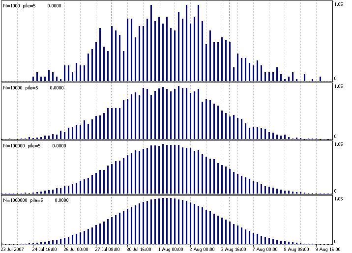
Fig.1. Indicator that creates a normal distribution of a uniform one.

Here, N means how many times we took the average of pile=5 uniformly distributed numbers on the interval of 0 to 100. We obtained four charts, very similar in appearance. If we normalize them somehow at the limit (adjunct to a single scale), we will obtain a several realizations of the standard normal distribution. The only fly in this ointment is that pricing on financial markets (to be more exact, price increments and other derivatives of those increments), generally speaking, does not fit into the normal distribution. The probability of a rather rare event (for example, of price decreasing by 50%) on financial markets is, whereas low, but still considerably higher than at normal distribution. This is why one should remember this when estimating risks on the basis of normal distribution.

Quantity Transforms into Quality

Even this simple example of modelling normal distribution shows that the amount of data to be processed counts for much. The more initial data there are, the more precise and valid the result is. The smallest number in the sample is considered to have to exceed 30. It means that, if we want to estimate results of trades (for example, an Expert Advisor in the Tester), the amount of trades below 30 is insufficient to make statistically reliable conclusions about some parameters of the system. The more trades we analyze, the less the probability is that these trades are just happily snatched elements of a not very reliable trading system. Hence, the final profit in a series of 150 trades affords more grounds for putting the system into service than a system estimated on only 15 trades.

Mathematical Expectation and Dispersion as Risk Estimate

The two most important characteristics of a distribution are mathematical expectation (average) and dispersion. The standard normal distribution has a mathematical expectation equal to zero. At that, the distribution center is located at zero, as well. Flatness or steepness of normal distribution is characterized by the measure of spread of a random value within the mathematical expectation area. It is dispersion that shows us how values are spread about the random value's mathematical expectation.

Mathematical expectation can be found in a very simple way: For countable sets, all distribution values are summed up, the obtained sum being divided by the amount of values. For example, a set of natural numbers is infinite, but countable, since each value can be collated with its index (order number). For uncountable sets, integration will be applied. To estimate mathematical expectation of a series of trades, we will sum up all trade results and divide the obtained amount by the amount of trades. The obtained value will show the expected average result of each trade. If mathematical expectation is positive, we profit in average. If it is negative, we lose in average.

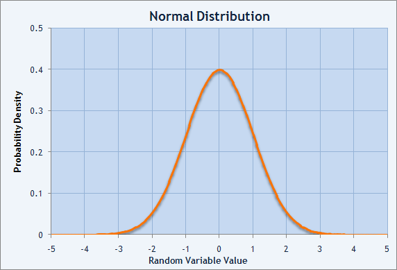
Fig.2. Chart of probability density of normal distribution.

The measure of spread of the distribution is the sum of squared deviations of the random value from its mathematical expectation. This characteristic of the distribution is called dispersion. Normally, mathematical expectation for a randomly distributed value is named M(X). Then dispersion may be described as D(X) = M((X-M(X))^2 ). The square root of dispersion is named standard deviation. It is also defined as sigma (σ). It is a normal distribution having mathematical expectation equal to zero and standard deviation equal to 1 that is named normal, or Gaussian, distribution.

The higher the value of standard deviation is, the more changeable the trading capital is, the higher its risk is. If the mathematical expectation is positive (a profitable strategy) and equal to $100 and if the standard deviation is equal to $500, we risk a sum, which is several times larger, to earn each dollar. For example, we have the results of 30 trades:

Trade Number X (Result) 1 -17.08 2 -41.00 3 147.80 4 -159.96 5 216.97 6 98.30 7 -87.74 8 -27.84 9 12.34 10 48.14 11 -60.91 12 10.63 13 -125.42 14 -27.81 15 88.03		Trade Number X (Result) 16 32.93 17 54.82 18 -160.10 19 -83.37 20 118.40 21 145.65 22 48.44 23 77.39 24 57.48 25 67.75 26 -127.10 27 -70.18 28 -127.61 29 31.31 30 -12.55

 

To find the mathematical expectation for this sequence of trades, let us sum up all the results and divide this by 30. We will obtain mean value M(X) equal to $4.26. To find the standard deviation, let us subtract the average from each trade's result, square it, and find the sum of squares. The obtained value will be divided by 29 (the amount of trades minus one). So we will obtain dispersion D equal to 9 353.623. Having generated square root of the dispersion, we obtain standard deviation, sigma, equal to $96.71.

The check data are given in the table below:

Trade Number	X (Result)	X-M(X) (Difference)	(X-M(X))^2 (Square of Difference)
1	-17.08	-21.34	455.3956
2	-41.00	-45.26	2 048.4676
3	147.80	143.54	20 603.7316
4	-159.96	-164.22	26 968.2084
5	216.97	212.71	45 245.5441
6	98.30	94.04	8 843.5216
7	-87.74	-92.00	8 464.00
8	-27.84	-32.10	1 030.41
9	12.34	8.08	65.2864
10	48.14	43.88	1 925.4544
11	-60.91	-65.17	4 247.1289
12	10.63	6.37	40.5769
13	-125.42	-129.68	16 816.9024
14	-27.81	-32.07	1 028.4849
15	88.03	83.77	7 017.4129
16	32.93	28.67	821.9689
17	54.82	50.56	2 556.3136
18	-160.10	-164.36	27 014.2096
19	-83.37	-87.63	7 679.0169
20	118.40	114.14	13 027.9396
21	145.65	141.39	19 991.1321
22	48.44	44.18	1 951.8724
23	77.39	73.13	5 347.9969
24	57.48	53.22	2 832.3684
25	67.75	63.49	4 030.9801
26	-127.10	-131.36	17 255.4496
27	-70.18	-74.44	5 541.3136
28	-127.61	-131.87	17 389.6969
29	31.31	27.05	731.7025
30	-12.55	-16.81	282.5761

 

What we have obtained is the mathematical expectation equal to $4.26 and standard deviation of $96.71. It is not the best ratio between the risk and the average trade. Profit chart below confirms this:

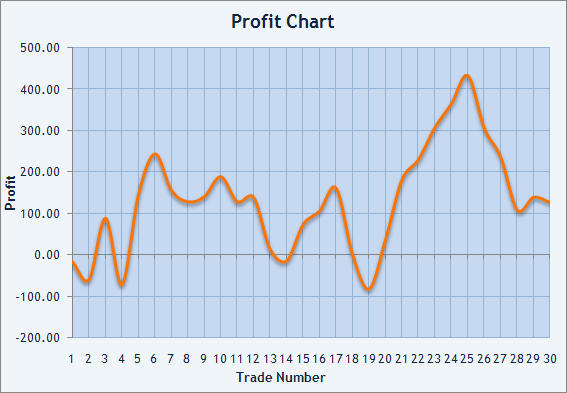
Fig.3. Balance graph for trades made.

Do I Trade Randomly? Z-Score

The assumption itself that profit gained as a result of a series of trades is random sounds sardonically for the most of traders. Having spent a lot of time searching for a successful trading system and observed that the system found has already resulted in some real profits on a rather limited period of time, the trader supposes to have found a proper approach to the market. How can he or she assume that all this was just a randomness? That's a bit too thick, especially for newbies. Nevertheless, it is essential to estimate the results objectively. In this case, normal distribution, again, comes to the rescue.

We don't know what there will be each trade's result. We can only say that we either gain profit (+) or meet with losses (-). Profits and losses alternate in different ways for different trading systems. For example, if the expected profit is 5 times less than the expected loss at triggering of Stop Loss, it would be reasonable to presume that profitable trades (+ trades) will significantly prevail over the losing ones (- trades). Z-Score allows us to estimate how often profitable trades are alternated with losing ones.

Z for a trading system is calculated by the following formula:

Z=(N*(R-0.5)-P)/((P*(P-N))/(N-1))^(1/2) where: N - total amount of trades in a series; R - total amount of series of profitable and losing trades; P = 2*W*L; W - total amount of profitable trades in the series; L - total amount of losing trades in the series.

 

A series is a sequence of pluses followed by each other (for example, +++) or minuses followed by each other (for example, --). R counts the amount of such series.

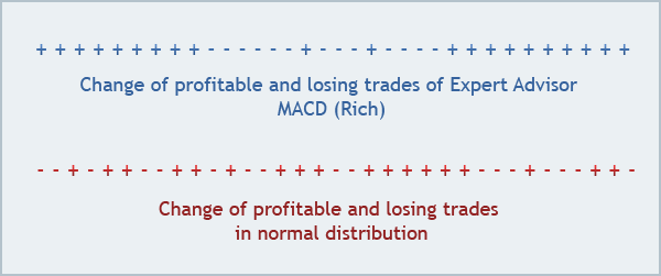
Fig.4. Comparison of two series of profits and losses.

In Fig. 4, a part of the sequence of profits and losses of the Expert Advisor that took the first place at the Automated Trading Championship 2006 is shown in blue. Z-score of its competition account has the value of -3.85, probability of 99.74% is given in brackets. This means that, with a probability of 99.74%, trades on this account had a positive dependence between them (Z-score is negative): a profit was followed by a profit, a loss was followed by a loss. Is this the case? Those who were watching the Championship would probably remember that Roman Rich placed his version of Expert Advisor MACD that had frequently opened three trades running in the same direction.

A typical sequence of positive and negative values of the random value in normal distribution is shown in red. We can see that these sequences differ. However, how can we measure this difference? Z-score answer this question: Does your sequence of profits and losses contain more or fewer strips (profitable or losing series) than you can expect for a really random sequence without any dependence between trades? If the Z-score is close to zero, we cannot say that trades distribution differs from normal distribution. Z-score of a trading sequence may inform us about possible dependence between consecutive trades.

At that, the values of Z are interpreted in the same way as the probability of deviation from zero of a random value distributed according to the standard normal distribution (average=0, sigma=1). If the probability of falling a normally distributed random value within the range of ±3σ is 99.74%, the falling of this value outside of this interval with the same probability of 99.74% informs us that this random value does not belong to this given normal distribution. This is why the "3-sigma rule'' is read as follows: a normal random value deviates from its average by no more than 3-sigma distance.

Sign of Z informs us about the type of dependence. Plus means that it is most probably that the profitable trade will be followed by a losing one. Minus says that the profit will be followed by a profit, a loss will be followed by a loss again. A small table below illustrates the type and the probability of dependence between trades as compared to normal distribution.

Z-Score	Probability of Dependence, %	Type of Dependence
-3	99.73	Positive
-2.9	99.63	Positive
-2.8	99.49	Positive
-2.7	99.31	Positive
-2.6	99.07	Positive
-2.5	98.76	Positive
-2	95.45	Positive
-1.5	86.64	Indeterminate
-1.0	68.27	Indeterminate
0.0	0.00	Indeterminate
1.0	68.27	Indeterminate
1.5	86.64	Indeterminate
2.0	95.45	Negative
2.5	98.76	Negative
2.6	99.07	Negative
2.7	99.31	Negative
2.8	99.49	Negative
2.9	99.63	Negative
3.0	99.73	Negative

 

A positive dependence between trades means that a profit will cause a new profit, whereas a loss will cause a new loss. A negative dependence means that a profit will be followed by a loss, whereas the loss will be followed by a profit. The dependence found allows us to regulate sizes of positions to be opened (ideally) or even skip some of them and open them only virtually in order to watch trade sequences.

Holding Period Returns (HPR)

In his book, The Mathematics of Money Management, Ralph Vince uses the notion of HPR (holding period returns). A trade resulted in profit of 10% has the HPR=1+0.10=1.10. A trade resulted in a loss of 10% has the HPR=1-0. 10=0.90. You can also obtain the value of HPR for a trade by dividing the balance value after the trade has been closed (BalanceClose) by the balance value at opening of the trade (BalanceOpen). HPR=BalanceClose/BalanceOpen. Thus, every trade has both a result in money terms and a result expressed as HPR. This will allow us to compare systems independently on the size of traded contracts. One of indexes used in such comparison is the arithmetic average, AHPR (average holding period returns).

To find the AHPR, we should sum up all the HPRs and divide the result by the amount of trades. Let's consider these calculations using the above example of 30 trades. Suppose we started trading with $500 on the account. Let's make a new table:

Trade Number	Balance, $	Result, $	Balance at Close, $	HPR
1	500.00	-17.08	482.92	0.9658
2	482.92	-41.00	441.92	0.9151
3	441.92	147.8	589.72	1.3344
4	589.72	-159.96	429.76	0.7288
5	429.76	216.97	646.73	1.5049
6	646.73	98.30	745.03	1.1520
7	745.03	-87.74	657.29	0.8822
8	657.29	-27.84	629.45	0.9576
9	629.45	12.34	641.79	1.0196
10	641.79	48.14	689.93	1.0750
11	689.93	-60.91	629.02	0.9117
12	629.02	10.63	639.65	1.0169
13	639.65	-125.42	514.23	0.8039
14	514.23	-27.81	486.42	0.9459
15	486.42	88.03	574.45	1.1810
16	574.45	32.93	607.38	1.0573
17	607.38	54.82	662.20	1.0903
18	662.20	-160.10	502.10	0.7582
19	502.10	-83.37	418.73	0.8340
20	418.73	118.4	537.13	1.2828
21	537.13	145.65	682.78	1.2712
22	682.78	48.44	731.22	1.0709
23	731.22	77.39	808.61	1.1058
24	808.61	57.48	866.09	1.0711
25	866.09	67.75	933.84	1.0782
26	933.84	-127.10	806.74	0.8639
27	806.74	-70.18	736.56	0.9130
28	736.56	-127.61	608.95	0.8267
29	608.95	31.31	640.26	1.0514
30	640.26	-12.55	627.71	0.9804

 

AHPR will be found as the arithmetic average. It is equal to 1.0217. In other words, we averagely earn (1.0217-1)*100%=2.17% on each trade. Is this the case? If we multiply 2.17 by 30, we will see that the income should make 65.1%. Let's multiply the initial amount of $500 by 65.1% and obtain $325.50. At the same time, the real profit makes (627.71-500)/500*100%=25.54%. Thus, the arithmetic average of HPR does not always allow us to estimate a system properly.

Along with arithmetic average, Ralph Vince introduces the notion of geometric average that we shall call GHPR (geometric holding period returns), which is practically always less than the AHPR. The geometric average is the growth factor per game and is found by the following formula:

GHPR=(BalanceClose/BalanceOpen)^(1/N) where: N - amount of trades; BalanceOpen - initial state of the account; BalanceClose - final state of the account.

 

The system having the largest GHPR will make the highest profits if we trade on the basis of reinvestment. The GHPR below one means that the system will lose money if we trade on the basis of reinvestment. A good illustration of the difference between AHPR and GHPR can be sashken's account history. He was the Championship's leader for a long time. AHPR=9.98% impresses, but the final GHPR=-27.68% puts everything into perspective.

Sharpe Ratio

Efficiency of investments is often estimated in terms of profits dispersion. One of such indexes is Sharpe Ratio. This index shows how AHPR decreased by the risk-free rate (RFR) relates to standard deviation (SD) of the HPR sequence. The value of RFR is usually taken as equal to interest rate on deposit in the bank or interest rate on treasury obligations. In our example, AHPR=1.0217, SD(HPR)=0.17607, RFR=0.

Sharpe Ratio=(AHPR-(1+RFR))/SD where: AHPR - average holding period returns; RFR - risk-free rate; SD - standard deviation.

 

Sharpe Ratio=(1.0217-(1+0))/0.17607=0.0217/0.17607=0.1232. For normal distribution, over 99% of random values are within the range of ±3σ (sigma=SD) about the mean value M(X). It follows that the value of Sharpe Ratio exceeding 3 is very good. In Fig. 5 below, we can see that, if the trade results are distributed normally and Sharpe Ratio=3, the probability of losing is below 1% per trade according to 3-sigma rule.

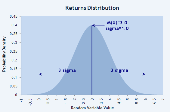
Fig.5. Normal distribution of trade results with the losing probability of less than 1%.

The account of Participant named RobinHood confirms this: his EA made 26 trades at the Automated Trading Championship 2006 without any losing one among them. Sharpe Ratio=3.07!

Linear Regression (LR) and Coefficient of Linear Correlation (CLC)

There is also another way to estimate trade results stability. Sharpe Ratio allows us to estimate the risk the capital is running, but we can also try to estimate the balance curve smooth degree. If we impose the values of balance at closing of each trade, we will be able to draw a broken line. These points can be fitted with a certain straight line that will show us the mean direction of capital changes. Let us consider an example of this opportunity using the balance graph of Expert Advisor Phoenix_4 developed by Hendrick.

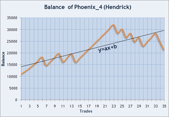
Fig. 6. Balance graph of Hendrick, the Participant of the Automated Trading Championship 2006.

We have to find such coefficients a and b that this line goes as close as possible to the points being fitted. In our case, x is the trade number, y is the balance value at closing the trade.

x (trades) y (balance) 1 11 069.50 2 12 213.90 3 13 533.20 4 14 991.90 5 16 598.10 6 18 372.80 7 14 867.50 8 16 416.80 9 18 108.30 10 19 873.60 11 16 321.80 12 17 980.40 13 19 744.50 14 16 199.00 15 17 943.20 16 19 681.00 17 21 471.00 18 23 254.90		x (trades) y (balance) 19 24 999.40 20 26 781.60 21 28 569.50 22 30 362.00 23 32 148.20 24 28 566.70 25 30 314.10 26 26 687.80 27 28 506.70 28 24 902.20 29 26 711.60 30 23 068.00 31 24 894.10 32 26 672.40 33 28 446.30 34 24 881.60 35 21 342.60

 

Coefficients of an approximating straight are usually found by least squares method (LS method). Suppose we have this straight with known coefficients a and b. For every x, we have two values: y(x)=a*x+b and balance(x). Deviation of balance(x) from y(x) will be denoted as d(x)=y(x)-balance(x). SSD (sum of squared deviations) can be calculated as SD=Summ{d(n)^2}. Finding the straight by LS method means searching for such a and b that SD is minimal. This straight is also named linear regression(LR) for the given sequence.

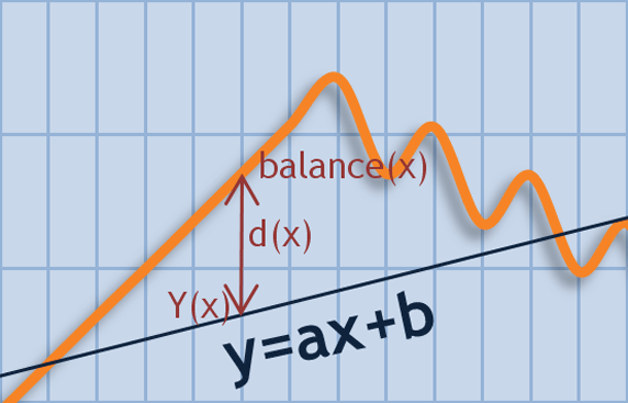
Fig. 7. Balance value deviation from the straight of y=ax+b

Having obtained coefficients of the straight of y=a*x+b using the LS method, we can estimate the balance value deviation from the found straight in money terms. If we calculate the arithmetic average for sequence d(x), we will be certain that М(d(x)) is close to zero (to be more exact, it is equal to zero to some calculation accuracy degree). At the same time, the SSD of SD is not equal to zero and has a certain limited value. The square root of SD/(N-2) shows the spread of values in the Balance graph about the straight line and allows to estimate trading systems at identical values of the initial state of the account. We will call this parameter LR Standard Error.

Below are values of this parameter for the first 15 accounts in the Automated Trading Championship 2006:

#	Login	LR Standard Error, $	Profit, $
1	Rich	6 582.66	25 175.60
2	ldamiani	5 796.32	15 628.40
3	GODZILLA	2 275.99	11 378.70
4	valvk	3 938.29	9 819.40
5	Hendrick	3 687.37	9 732.30
6	bvpbvp	9 208.08	8 236.00
7	Flame	2 532.58	7 676.20
8	Berserk	1 943.72	7 383.70
9	vgc	905.10	6 801.30
10	RobinHood	109.11	5 643.10
11	alexgomel	763.76	5 557.50
12	LorDen	1 229.40	5 247.90
13	systrad5	6 239.33	5 141.10
14	emil	2 667.76	4 658.20
15	payday	1 686.10	4 588.90

 

However, the degree of approximation of the balance graph to a straight can be measured in both money terms and absolute terms. For this, we can use correlation rate. Correlation rate, r, measures the degree of correlation between two sequences of numbers. Its value may lie within the range of -1 to +1. If r=+1, it means that two sequences have identical behavior and the correlation is positive.

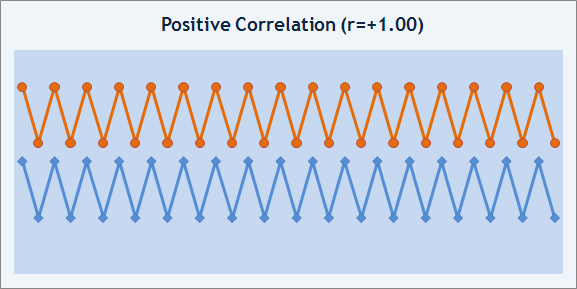
Fig. 8. Positive correlation example.

If r=-1, the two sequences change in opposition, the correlation is negative.

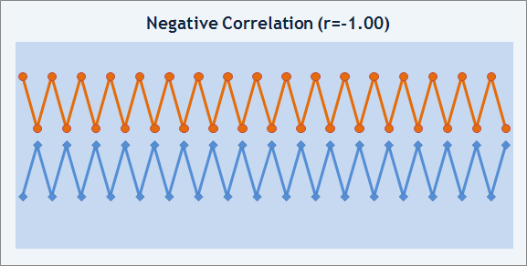
Fig. 9. Negative correlation example.

If r=0, it means that there is no dependence found between the sequences. It should be emphasized that r=0 does not mean that there is no correlation between the sequences, it just says that such a correlation has not been found. This must be remembered. In our case, we have to compare two sequences of numbers: one sequence from the balance graph and the other sequence representing the appropriate points along the linear regression line.

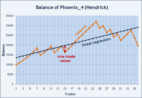
Fig. 10. Values of balance and points on linear regression.

Below is the table representation of the same data:

Trade Balance Regression Line 0 10 000.00 13 616.00 1 11 069.52 14 059.78 2 12 297.35 14 503.57 3 13 616.65 14 947.36 4 15 127.22 15 391.14 5 16 733.41 15 834.93 6 18 508.11 16 278.72 7 14 794.02 16 722.50 8 16 160.14 17 166.29 9 17 784.79 17 610.07 10 19 410.98 18 053.86 11 16 110.02 18 497.65 12 17 829.19 18 941.43 13 19 593.30 19 385.22 14 16 360.33 19 829.01 15 18 104.55 20 272.79 16 19 905.68 20 716.58 17 21 886.31 21 160.36			Trade Balance Regression Line 18 23 733.76 21 604.15 19 25 337.77 22 047.94 20 27 183.33 22 491.72 21 28 689.30 22 935.51 22 30 411.32 23 379.29 23 32 197.49 23 823.08 24 28 679.11 24 266.87 25 29 933.86 24 710.65 26 26 371.61 25 154.44 27 28 118.95 25 598.23 28 24 157.69 26 042.01 29 25 967.10 26 485.80 30 22 387.85 26 929.58 31 24 070.10 27 373.37 32 25 913.20 27 817.16 33 27 751.84 28 260.94 34 23 833.08 28 704.73 35 19 732.31 29 148.51

 

Let's denote balance values as X and the sequence of points on the straight regression line as Y. To calculate the coefficient of linear correlation between sequences X and Y, it is necessary to find mean values M(X) and M(Y) first. Then we will create a new sequence T=(X-M(X))*(Y-M(Y)) and calculate its mean value as M(T)=cov(X, Y)=M((X-M(X))*(Y-M(Y))). The found value of cov(X,Y) is named covarianceof X and Y and means mathematical expectation of product (X-M(X))*(Y-M(Y)). For our example, covariance value is 21 253 775.08. Please note that M(X) and M(Y) are equal and have the value of 21 382.26 each. It means that the Balance mean value and the average of the fitting straight are equal.

T=(X-M(X))*(Y-M(Y)) M(T)=cov(X,Y)=M((X-M(X))*(Y-M(Y))) where: X - Balance; Y - linear regression; M(X) - Balance mean value; M(Y) - LR mean value.

 

The only thing that remains to be done is calculation of Sx and Sy. To calculate Sx, we will find the sum of values of (X-M(X))^2, i.e., find the SSD of X from its mean value. Remember how we calculated dispersion and the algorithm of LS method. As you can see they are all related. The found SSD will be divided by the amount of numbers in the sequence - in our case, 36 (from zero to 35) - and extract the square root of the resulting value. So we have obtained the value of Sx. The value of Sy will be calculated in the same way. In our example, Sx=5839. 098245 and Sy=4610. 181675.

Sx=Summ{(X-M(X))^2}/N Sy=Summ{(Y-M(Y))^2}/N r=cov(X,Y)/(Sx* Sy) where: N - amount of trades; X - Balance; Y - linear regression; M(X) - Balance mean value; M(Y) - LR mean value.

 

Now we can find the value of correlation coefficient as r=21 253 775.08/(5839. 098245*4610. 181675)=0.789536583. This is below one, but far from zero. Thus, we can say that the balance graph correlates with the trend line valued as 0.79. By comparison to other systems, we will gradually learn how to interpret the values of correlation coefficient. At page "Reports" of the Championship, this parameter is named LR correlation. The only difference made to calculate this parameter within the framework of the Championship is that the sign of LR correlation indicates the trade profitability.

The matter is that we could calculate the coefficient of correlation between the balance graph and any straight. For purposes of the Championship, it was calculated for ascending trend line, hence, if LR correlation is above zero, the trading is profitable. If it is below zero, it is losing. Sometimes an interesting effect occurs where the account shoes profit, but LR correlation is negative. This can mean that trading is losing, anyway. An example of such situation can be seen at Aver's. The Total Net Profit makes $2 642, whereas LR сorrelation is -0.11. There is likely no correlation, in this case. It means we just could not judge about the future of the account.

MAE and MFE Will Tell Us Much

We are often warned: "Cut the losses and let profit grow". Looking at final trade results, we cannot draw any conclusions about whether protective stops (Stop Loss) are available or whether the profit fixation is effective. We only see the position opening date, the closing date and the final result - a profit or a loss. This is like judging about a person by his or her birth and death dates. Without knowing about floating profits during every trade's life and about all positions as a total, we cannot judge about the nature of the trading system. How risky is it? How was the profit reached? Was the paper profit lost? Answers to these questions can be rather well provided by parameters MAE (Maximum Adverse Excursion) and MFE (Maximum Favorable Excursion).

Every open position (until it is closed) continuously experiences profit fluctuations. Every trade reached its maximal profit and its maximal loss during the period between its opening and closing. MFE shows the maximal price movement in a favorable direction. Respectively, MAE shows the maximal price movement in an adverse direction. It would be logical to measure both indexes in points. However, if different currency pairs were traded,we will have to express it in money terms.

Every closed trade corresponds to its result (return) and two indexes - MFE and MAE. If the trade resulted in profit of $100, MAE reaching -$1000, this does not speak for this trade's best. Availability of many trades resulted in profits, but having large negative values of MAE per trade, informs us that the system just "sits out" losing positions. Such trading is fated to failure sooner or later.

Similarly, values of MFE can provide some useful information. If a position was opened in a right direction, MFE per trade reached $3000, but the trade was then closed resulting in the profit of $500, we can say that it would be good to elaborate the system of unfixed profit protection. This may be Trailing Stop that we can move after the price if the latter one moves in a favorable direction. If short profits are systematic, the system can be significantly improved. MFE will tell us about this.

For visual analysis to be more convenient, it would be better to use graphical representation of distribution of values of MAE and MFE. If we impose each trade into a chart, we will see how the result has been obtained. For example, if we have another look into "Reports" of RobinHood who didn't have any losing trades at all, we will see that each trade had a drawdown (MAE) from -$120 to -$2500.

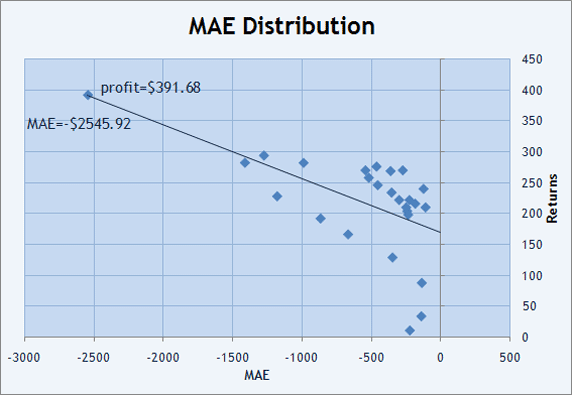
Fig. 11. Trades distribution on the plane of MAExReturns

Besides, we can draw a straight line to fit the Returns x MAE distribution using the LS method. In Fig. 11, it is shown in red and has a negative slope (the straight values decrease when moving from left to right). Parameter Correlation(Profits, MAE)=-0.59 allows us to estimate how close to the straight the points are distributed in the chart. Negative value shows negative slope of the fitting line.

If you look through other Participants' accounts, you will see that correlation coefficient is usually positive. In the above example, the descending slope of the line says us that it tends to get more and more drawdowns in order not to allow losing trades. Now we can understand what price has been paid for the ideal value of parameter LR Correlation=1!

Similarly, we can build a graph of distribution of Returns and MFE, as well as find the values of Correlation(Profits, MFE)=0.77 and Correlation(MFE, MAE)=-0.59. Correlation(Profits, MFE) is positive and tends to one (0.77). This informs us that the strategy tries not to allow long "sittings out" floating profits. It is more likely that the profit is not allowed to grow enough and trades are closed by Take Profit. As you can see, distributions of MAE and MFE дgive us a visual estimate and values of Correlation(Profits, MFE) and Correlation(Profits, MAE) can inform us about the nature of trading, even without charts.

Values of Correlation(MFE, MAE), Correlation(NormalizedProfits, MAE) and Correlation(NormalizedProfits, MFE) in the Championship Participants' "Reports" are given as additional information.

Trade Result Normalization

In development of trading systems, they usually use fixed sizes for positions. This allows easier optimization of system parameters in order to find those more optimal on certain criteria. However, after the inputs have been found, the logical question occurs: What sizing management system (Money Management, MM) should be applied. The size of positions opened relates directly to the amount of money on the account, so it would not be reasonable to trade on the account with $5 000 in the same way as on that with $50 000. Besides, an ММ system can open positions, which are not directly proportional. I mean a position opened on the account with $50 000 should not necessarily be 10 times more than that opened on a $5 000 deposit.

Position sizes may also vary according to the current market phase, to the results of the latest several trades analysis, and so on. So the money-management system applied can essentially change the initial appearance of a trading system. How can we then estimate the impact of the applied money-management system? Was it useful or did it just worsen the negative sides of our trading approach? How can we compare the trade results on several accounts having the same deposit size at the beginning? A possible solution would be normalization of trade results.

NP=TradeProfit/TradeLots*MinimumLots where: TradeProfit - profit per trade in money terms; TradeLots - position size (lots); MinimumLots - minimum allowable position size.

 

Normalization will be realized as follows: We will divide each trade's result (profit or loss) by the position volume and then multiply by the minimum allowable position size. For example, order #4399142 BUY 2.3 lots USDJPY was closed with the profit of $4 056. 20 + $118.51 (swaps) = $4 174.71. This example was taken from the account of GODZILLA (Nikolay Kositsin). Let's divide the result by 2.3 and multiply by 0.1 (the minimum allowable position size), and obtain a profit of $4 056.20/2.3 * 0.1 = $176.36 and swaps = $5.15. these would be results for the order of 0.1-lot size. Let us do the same with results of all trades and we will then obtain Normalized Profits (NP).

the first thing we think about is finding values of Correlation(NormalizedProfits, MAE) and Correlation(NormalizedProfits, MFE) and comparing them to the initial Correlation(Profits, MAE) and Correlation(Profits, MFE). If the difference between parameters is significant, the applied method has likely changed the initial system essentially. They say that applying of ММ can "kill" a profitable system, but it cannot turn a losing system into a profitable one. in the Championship, the account of TMR is a rare exception where changing Correlation(NormalizedProfits, MFE) value from 0.23 to 0.63 allowed the trader to "close in black".

How Can We Estimate the Strategy's Aggression?

We can benefit even more from normalized trades in measuring of how the MM method applied influences the strategy. It is obvious that increasing sizes of positions 10 times will cause that the final result will differ from the initial one 10 times. And what if we change the trade sizes not by a given number of times, but depending on the current developments? Results obtained by trust-managing companies are usually compared to a certain model, usually - to a stock index. Beta Coefficient shows by how many times the account deposit changes as compared to the index. If we take normalized trades as an index, we will be able to know how much more volatile the results became as compared to the initial system (0.1-lot trades).

Thus, first of all, we calculate covariance - cov(Profits, NormalizedProfits). then we calculate the dispersion of normalized trades naming the sequence of normalized trades as NP. For this, we will calculate the mathematical expectation of normalized trades named M(NP). M(NP) shows the average trade result for normalized trades. Then we will find the SSD of normalized trades from M(NP), i.e., we will sum up (NP-M(NP))^2. The obtained result will be then divided by the amount of trades and name D(NP). This is the dispersion of normalized trades. Let's divide covariance between the system under measuring, Profits, and the ideal index, NormalizedProfits cov(Profits, NormalizedProfits), by the index dispersion D(NP). The result will be the parameter value that will allow us to estimate by how many times more volatile the capital is than the results of original trades (trades in the Championship) as compared to normalized trades. This parameter is named Money Compounding in the "Reports". It shows the trading aggression level to some extent.

MoneyCompounding=cov(Profits, NP)/D(NP)= M((Profits-M(Profits))*(NP-M(NP)))/M((NP-M(NP))^2) where: Profits - trade results; NP - normalized trade results; M(NP) - mean value of normalized trades.

 

Now we can revise the way we read the table of Participants of the Automated Trading Championship 2006:

#	Login	LR Standard error, $	LR Correlation	Sharpe	GHPR	Z-score (%)	Money Compounding	Profit, $
1	Rich	6 582.66	0.81	0.41	2.55	-3.85(99.74)	17.27	25 175.60
2	ldamiani	5 796.32	0.64	0.21	2.89	-2.47 (98.65)	28.79	15 628.40
3	GODZILLA	2 275.99	0.9	0.19	1.97	0.7(51.61)	16.54	11 378.70
4	valvk	3 938.29	0.89	0.22	1.68	0.26(20.51)	40.17	9 819.40
5	Hendrick	3 687.37	0.79	0.24	1.96	0.97(66.8)	49.02	9 732.30
6	bvpbvp	9 208.08	0.58	0.43	12.77	1.2(76.99)	50.00	8 236.00
7	Flame	2 532.58	0.75	0.36	3.87	-2.07(96.06)	6.75	7 676.20
8	Berserk	1 943.72	0.68	0.20	1.59	0.69(50.98)	17.49	7 383.70
9	vgc	905.10	0.95	0.29	1.63	0.58(43.13)	8.06	6 801.30
10	RobinHood	109.11	1.00	3.07	1.74	N/A (N/A)	41.87	5 643.10
11	alexgomel	763.76	0.95	0.43	2.63	1.52(87.15)	10.00	5 557.50
12	LorDen	1229.40	0.8	0.33	3.06	1.34(81.98)	49.65	5 247.90
13	systrad5	6 239.33	0.66	0.27	2.47	-0.9(63.19)	42.25	5 141.10
14	emil	2 667.76	0.77	0.21	1.93	-1.97(95.12)	12.75	4 658.20
15	payday	1686.10	0.75	0.16	0.88	0.46(35.45)	10.00	4 588.90

 

The LR Standard error in Winners' accounts was not the smallest. At the same time, the balance graphs of the most profitable Expert Advisors were rather smooth since the LR Correlation values are not far from 1.0. The Sharpe Ratio lied basically within the range of 0.20 to 0.40. The only EA with extremal Sharpe Ratio=3.07 turned not to have very good values of MAE and MFE.

The GHPR per trade is basically located within the range from 1.5 to 3%. At that, the Winners did not have the largest values of GHPR, though not the smallest ones. Extreme value GHPR=12.77% says us again that there was an abnormality in trading, and we can see that this account experienced the largest fluctuations with LR Standard error=$9 208.08.

Z-score does not give us any generalizations about the first 15 Championship Participants, but values of |Z|>2.0 may draw our attention to the trading history in order to understand the nature of dependence between trades on the account. Thus, we know that Z=-3.85 for Rich's account was practically reached due to simultaneous opening of three positions. And how are things with ldamiani's account?

Finally, the last column in the above table, Money Compounding, also has a large range of values from 8 to 50, 50 being the maximal value for this Championship since the maximal allowable trade size made 5.0 lots, which is 50 times more than the minimal size of 0.1 lot. However, curiously enough, this parameter is not the largest at Winners. The Top Three's values are 17.27, 28.79 and 16.54. Did not the Winners fully used the maximal allowable position size? Yes, they did. the matter is, perhaps, that the MM methods did not considerably influence trading risks at general increasing of contract sizes. This is a visible evidence of that money management is very important for a trading system.

The 15th place was taken by payday. The EA of this Participant could not open trades with the size of more than 1. 0 lot due to a small error in the code. What if this error did not occur and position sizes were in creased 5 times, up to 5.0 lots? Would then the profit increase proportionally, from $4 588.90 to $22 944.50? Would the Participant then take the second place or would he experience an irrecoverable DrawDown due to increased risks? Would alexgomel be on the first place? His EA traded with only 1.0-лот trades, too. Or could vgc win, whose Expert Advisor most frequently opened trades of the size of less than 1.0 lot. All three have a good smooth balance graph. As you can see, the Championship's plot continues whereas it was over!

Conclusion: Don't Throw the Baby Out with the Bathwater

Opinions differ. This article gives some very general approaches to estimation of trading strategies. One can create many more criteria to estimate trade results. Each characteristic taken separately will not provide a full and objective estimate, but taken together they may help us to avoid lopsided approach in this matter.

We can say that we can subject to a "cross-examination" any positive result (a profit gained on a sufficient sequence of trades) in order to detect negative points in trading. This means that all these characteristics do not so much characterize the efficiency of the given trading strategy as inform us about weak points in trading we should pay attention at, without being satisfied with just a positive final result - the net profit gained on the account.

Well, we cannot create an ideal trading system, every system has its benefits and implications. Estimation test is used in order not to reject a trading approach dogmatically, but to know how to perform further development of trading systems and Expert Advisors. In this regard, statistical data accumulated during the Automated Trading Championship 2006 would be a great support for every trader.