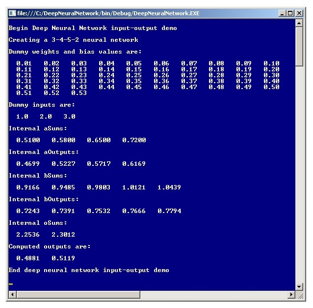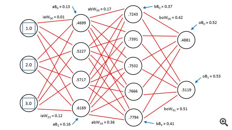
The term deep neural network can have several meanings, but one of the most common is to describe a neural network that has two or more layers of hidden processing neurons. This article explains how to create a deep neural network using C#. The best way to get a feel for what a deep neural network is and to see where this article is headed is to take a look at the demo program in Figure 1 and the associated diagram in Figure 2.
Both figures illustrate the input-output mechanism for a neural
network that has three inputs, a first hidden layer ("A") with four
neurons, a second hidden layer ("B") with five neurons and two outputs.
"There are several different meanings for exactly what a deep neural
network is, but one is just a neural network with two (or more) layers
of hidden nodes." 3-4-5-2 neural network requires a total of (3 * 4) + 4
+ (4 * 5) + 5 + (5 * 2) + 2 = 53 weights and bias values. In the demo,
the weights and biases are set to dummy values of 0.01, 0.02, . . . ,
0.53. The three inputs are arbitrarily set to 1.0, 2.0 and 3.0. Behind
the scenes, the neural network uses the hyperbolic tangent activation
function when computing the outputs of the two hidden layers, and the
softmax activation function when computing the final output values. The
two output values are 0.4881 and 0.5119.

Figure 1. Deep Neural Network Demo

Figure 2. Deep Neural Network Architecture
Research in the field of deep neural networks is relatively new compared to classical statistical techniques. The so-called Cybenko theorem states, somewhat loosely, that a fully connected feed-forward neural network with a single hidden layer can approximate any continuous function. The point of using a neural network with two layers of hidden neurons rather than a single hidden layer is that a two-hidden-layer neural network can, in theory, solve certain problems that a single-hidden-layer network cannot. Additionally, a two-hidden-layer neural network can sometimes solve problems that would require a huge number of nodes in a single-hidden-layer network.
This article assumes you have a basic grasp of neural network
concepts and terminology and at least intermediate-level programming
skills. The demo is coded using C#, but you should be able to refactor
the code to other languages such as JavaScript or Visual Basic .NET
without too much difficulty. Most normal error checking has been omitted
from the demo to keep the size of the code small and the main ideas as
clear as possible.
The Input-Output Mechanism
The input-output mechanism for a deep neural network with two hidden layers is best explained by example. Take a look at Figure 2.
Because of the complexity of the diagram, most of the weights and bias
value labels have been omitted, but because the values are sequential --
from 0.01 through 0.53 -- you should be able to infer exactly what the
unlabeled values are. Nodes, weights and biases are indexed (zero-based)
from top to bottom. The first hidden layer is called layer A in the
demo code and the second hidden layer is called layer B. For example,
the top-most input node has index [0] and the bottom-most node in the
second hidden layer has index.
In the diagram, label iaW00 means, "input to layer A weight from
input node 0 to A node 0." Label aB0 means, "A layer bias value for A
node 0." The output for layer-A node is 0.4699 and is computed as
follows (first, the sum of the node's inputs times associated with their
weights is computed):
(1.0)(0.01) + (2.0)(0.05) + (3.0)(0.09) = 0.38
Next, the associated bias is added:
0.38 + 0.13 = 0.51
Then, the hyperbolic tangent function is applied to the sum to give the node's local output value:
tanh(0.51) = 0.4699
The three other values for the layer-A hidden nodes are computed in the same way, and are 0.5227, 0.5717 and 0.6169, as you can see in both Figure 1 and Figure 2. Notice that the demo treats bias values as separate constants, rather than the somewhat confusing and common alternative of treating bias values as special weights associated with dummy constant 1.0-value inputs.
The output for layer-B node [0] is 0.7243. The node's intermediate sum is:
(0.4699)(0.17) + (0.5227)(0.22) + (0.5717)(0.27) + (0.6169)(0.32) = 0.5466
The bias is added:
0.5466 + 0.37 = 0.9166
And the hyperbolic tangent is applied:
tanh(0.9166) = 0.7243
The same pattern is followed to compute the other layer-B hidden node
values: 0.7391, 0.7532, 0.7666 and 0.7794. The values for final output
nodes [0] and [1] are computed in a slightly different way because
softmax activation is used to coerce the sum of the outputs to 1.0.
Preliminary (before activation) output [0] is:
(0.7243)(0.42) + (0.7391)(0.44) + (0.7532)(0.46) + (0.7666)(0.48) + (0.7794)(0.50) + 0.52 = 2.2536
Similarly, preliminary output is:
(0.7243)(0.43) + (0.7391)(0.45) + (0.7532)(0.47) + (0.7666)(0.49) + (0.7794)(0.51) + 0.53 = 2.3012

Applying softmax, final output [0] = exp(2.2536) / (exp(2.2536) + exp(2.3012)) = 0.4881.
And final output [1] = exp(2.3012) / (exp(2.2536) + exp(2.3012)) = 0.5119
The two final output computations are illustrated using the math definition of softmax activation. The demo program uses a derivation of the definition to avoid arithmetic overflow.


