Continuous Walk-Forward Optimization (Part 4): Optimization Manager (Auto Optimizer)

Introduction

This is the next article within the "Continuous Forward Optimization" series. Here, I present the created program, which implements the programmed automatic optimization. Previous articles described the details of program implementation both on terminal side and on the library side, which is used to work with the generated optimization reports. You can check out these articles at the below links:

1. Continuous Walk-Forward Optimization (Part 1): Working with optimization reports
2. Continuous Walk-Forward Optimization (Part 2): Mechanism for creating an optimization report for any robot
3. Continuous Walk-Forward Optimization (Part 3): Adapting a Robot to the Auto Optimizer

The current article demonstrates the general picture of the created product and serves as an instruction. The functionality of the created auto optimizer can be extended. Thus, the algorithm which we are going to discuss further can be easily replaced with your own optimizations algorithm allowing you to implement any desired idea. Also, further description discloses the internal structure of the created program. The main purpose of the article is to describe the mechanism of working with the resulting application and its capabilities. The fact is, my colleagues sometimes found it difficult to quickly understand it. However, the auto optimizer is quite easy to set up and use — and I will show this further. Thus, the article can be treated as an application usage instruction, which covers all possible pitfalls and setup specifics.

Auto Optimizer operation description

To proceed with the analysis of the created program we first need to define the purpose of this project. We decided to use a scientific approach in trading and started creating clearly programmed trading algorithms (no matter whether we deal with indicator-based robots or those applying fuzzy logic and neural networks — all of them are programmed algorithms that perform specific tasks). Therefore, the approach to the selection of optimization results should also be formalized. In other words, if during refuse to apply randomness in the trading process, then the process of preparation for trading should also be automated. Otherwise, we can select the results that we like randomly, which is closer to intuition than to the system trading. This idea is the first motive that encouraged me to create this application. The next one is the possibility to test algorithms by optimizing them — by using the Continuous Walk-Forward Optimization shown in the below figure.   

Continuous walk-forward optimization alternates between historical (yellow) and forward (green) optimization passes at a given time interval. Suppose you have a 10-year history. We determine that the optimization period should consist of an interval equal to 1 year, and a forward interval of 1 quarter (or 3 months). As a result, we have an interval equal to 1.25 years (1 year + 1 quarter) for one optimization pass + a forward test. In the figure, each line characterizes this time interval. 

Next, we produce the same type of process:

1. Optimize in the selected history period (1 year).
2. Select the best parameters among the results in the optimization interval, using a fixed method.
3. Shift to the forward time interval and run a test, get back to the first step — now on a shifted interval. Repeat until the current time period is reached.
4. Having collected testing results of each quarter, we obtain the final assessment of the algorithm viability.
5. The last optimization pass (for which there is no forward test) can be launched for trading.

Thus, we obtain a method for testing the sustainability of algorithms via optimization. However, in this case we must re-optimize the algorithms after every expiration of the forward period. In other words, we set a certain interval for the algorithm re-optimization, fix the methodology for selecting parameters and first perform this procedure on history, and later we repeat it every time the trading period which is equal to the forward test period expires. 

Firstly, this optimization technique allows us having a clearly defined optimization logic, which allows us to receive a result free from human intervention.

Secondly, by performing optimization on new assets or new algorithms using a similar technique, we get a complete picture of the stress tests of the algorithm. When both the parameter selection method and the optimized parameter are fixed and unchanged in all forward optimizations, we receive a continuous stress test, which will allow us to notice if the market becomes no longer suitable for our strategy.

Thirdly, we receive a lot of optimization frames within quite a small period, which increases the reliability of the performed tests. For example, with the above-mentioned division into a 1-year optimization and 1-quarter forward, a 2-year interval provides 4 stress tests and 1 final optimization.

Optimization launch setup

Now that we have discussed the process which the application executes, let's consider its usage. This series of articles is a logical continuation of my earlier articles about the graphical interface for the optimization process management:

1. Optimization management (Part I)
2. Optimization management (Part II)

The articles feature a description of how to run optimization or a test in the terminal as a controlled process. The same method is used in this series. However, one of the basic differences is that the controlling process is implemented not as an addition to the terminal, but as an independent program. This approach allows using all terminals installed on the computer. In the previous series of articles we created an extension which could be launched from a working terminal. The extension could use all the terminals installed on the computer in addition to the one from which it was launched. The current application also has access to all terminals installed on the computer, but it only works with one terminal at a time and it can launch any desired terminal.

To insure the successful operation of the auto optimizer, make sure the selected terminal is closed before you launch the app. 

The application operates as follows:

1. During the next process launch, no matter whether it is an optimization or a test, the application launches a terminal and delegates the entire testing process to the terminal. Once the test or optimization is complete, the terminal shuts down.
2. After the test or optimization, the robot generates a report with the optimization results (for more details please read the previous articles within this series).
3. The auto optimizer knows where the report is, so it reads and processes the report. Once processing is done, either a new optimization and testing stage is launched, or optimization is completed and the results are displayed in the "Result" tab. 

The implemented optimization mechanism will be considered later, while the purpose of the current part is to describe the program operation process with a minimum of technical details. Do not forget that you can add your own algorithm into the code part responsible for the optimization. The auto optimizer is a control program that starts optimization processes, but the logic of these processes can be different. Here is a screenshot of the main tab of the resulting application.

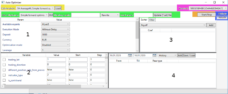
If you take a closer look at the screenshot, the first ComboBox called "Select Optimiser" and located in the green area, provides the selection of the optimization types implemented in the program. 

The application graphical interface is divided into 2 main tabs. The main tab is Settings. This is where we start working when we need to launch or stop optimization. The tab was described in detail in the second part. The other tab, "Result", is where optimization results are displayed.

First of all, when launching the auto optimizer, we need to select the terminal to be used. The terminal selection principle is the same as in the previous graphical interface used for optimization launch. In other words, the auto optimizer will find all terminals installed on this computer (however, only those that use a standard installation, and not a portable one). 

The "Settings" tab is divided into 4 sections. Borders of each screen part can be dragged. This is especially convenient when working with the algorithm having a lot of input parameters.

• The first part of the screen provides the list of parameters from the MetaTrader optimizer. The list of Expert Advisors "Available experts" is updated every time the selected terminal is changed. The list features all Expert Advisors located under the appropriate directory of the selected terminal. EAs are specified taking into account nested directories. 
• The second part of the screen contains the list of parameters of the selected algorithm. The list of parameters is found in appropriate files located in "MQL5/Profiles/Tester/{Expertname}.set". If there is no file for the selected EA, then after you select an EA in the first screen area, a terminal with a tester is opened first. Then the requested file is created with default settings. After that the terminal is closed. The list is changed every time you select another Expert Advisor from the "Available experts" list. If you wish to update the loaded list of parameters, simply click "Update (*.set) file", after that the list will be updated by opening the terminal and then closing it. Before this, the existing file will be deleted and a new file will be created under the same directory.
• The third part of the screen contains extremely important parameters: the list of filtering and sorting criteria for the array of unloaded data. The sorting procedure is discussed in detail in the first article within this series. As it was described in the first article, filtering criteria can be specified using ">=", "<=", "< || >", etc. 
• The fourth section of the screen contains a series of forward and historical time passes. The logics of the intervals was described above. Implementation of sorting and interaction between the passes were covered in the first article within this cycle. Pay attention that when launching a test not optimization (parameter Optimisation model = Disabled), this field should have either one historical time interval or two intervals (historical and forward). Since entering data during each auto optimizer start can be boring (verified by my own experience), a mechanism was implemented for saving data to a file. Upon a click on Save/Load, the availability of previously entered data in the list of parameters is checked. If the list is filled, save the received parameters to a file. If the list is empty, a file is selected from which a list with the dates of optimization passes will be loaded. The internal file structure will be described in further articles. Like all other files generated by the program, this one has xml format. Please note that the date entry format is "DD.MM.YYYY", while the data display format is "MM.DD.YYYY". This is because date is automatically converted into a string. This is not very critical to me, that is why I decided not to change this behavior.      

Also, because of the text format of set files we will not be able to distinguish between the formats of algorithm parameters. For example, all enum parameters are shown as int. That is why it was decided to display the list of parameters as strings in the second part of the screen. If it is not convenient for you to configure optimization steps and other robot parameters directly in the auto optimizer, you can perform all required settings in the terminal. Then after changing tabs in the tester (or after the terminal is closed) the settings will be written to the desired file. All you need to do is select the required algorithm in the auto optimizer — it will be loaded immediately with your settings.

Setting of the following fields is required for the launch of an optimization or a test from the auto optimizer:

1. Select EA.
2. Check the parameters to be optimized and select the range (just like in the terminal).
3. Select at least one sorting criterion: this will affect the sorting of data produced by the robot and the best of the results will be launched in the forward interval (can be omitted for a test run).
4. Select walk-forward optimization dates (or test dates if you run a test).   
5. Select the required optimizer if you run optimization ("Select Optimiser:" drop-down list). 
6. Specify "Asset name" — the name of the symbol for which the requested operation will be performed. In case of an error, the terminal will not be able to run the test or optimization.
7. You can use "Directory prefix" for the additional specification of the name of the optimization pass you are saving. A folder with the optimization results is created in a special internal program directory after the end of optimization. The folder name is set as follows: "{Directory prefix} {Selected optimiser} {Expert name} {Asset name}". These are the names shown in the "Optimisation:" list, from which they can be uploaded for viewing and further analysis.
8. Drop-down list with "Rewrite" or "Append" parameters is also optional. It sets the action to be performed by the auto optimizer if it finds results with the same name among the saved files. If "Rewrite" is selected, all files will be rewritten with new ones. If "Append" is selected, the matching optimization dates will be overwritten. If the same interval is found in current list of optimization intervals and in the list of previously saved ones, the saved results will be overwritten with the new ones. If the ranges are new, they will be added to existing ones.

Once the setup is performed, click "Start/Stop" to launch the process. A repeated click on this button will interrupt the optimization process. During the optimization process, its status is displayed in ProgressBar and in the text label which are located at the bottom of the auto optimizer window. After optimization end, the optimization results will be uploaded to the "Result" tab and ProgressBar will be reset to the initial state. However, if you run a test by clicking on "Start / Stop", the terminal will not be closed automatically. This is done for convenience and it allows the user to examine all required data. Once you have studied the required data, close the terminal manually to continue the auto optimizer operation. Please do not forget that the terminal should always be closed, because the application must be able to manage the terminal independently.

Also, you should configure the optimizer itself before launching optimizations. This is not a mandatory requirement, but the structure of the optimization manager allows creating custom optimizer as well as setting individual parameters for each of them. Settings can be opened by clicking on the "GUI" button located next to the combo box of optimizer selector. The settings of the implemented optimizer are as follows:

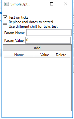
1. Test on ticks — indicates the method of data testing in historical and forward tests. The optimization method is specified in the first part of the "Settings" window, while the testing method is indicated in optimizer settings. If the option is enabled, testis will be performed using tick. If disabled, test will be performed in the OHLC 1 minute mode. 
2. Replace real dates to set — sets whether real optimization start and end dates should be replaced with the passed dates. Optimization beginning and end time is saved using a 1-minute timeframe. Sometimes, if there is no trading or it is a holiday, actual start and end dates can differ from the specified ones. If this option is enabled, the optimizer will set more familiar data and to know for sure to which interval the results belong. However, if you want to see real trading dates, uncheck the option.
3. Use different shift for tick test — we discussed in the second article that slippage and shift can be added to results. If ticks are used for testing, slippage can be disabled or totally reduced. This option was added exactly for this case. It is only activated when "Test on ticks" is enabled. To use the option, specify the algorithm parameters which are responsible for the indication of commission and slippage and set new values to them. By specifying the robot parameter responsible for slippage and setting it to 0 you can remove slippage from the results in the tick testing mode. After specifying a parameter and its value, add this parameter to the table via the "Add" parameter in order to save this parameter.

There is no need to save the entered parameters (there is no Save button), since they are saved automatically. Close this window before launching optimization to prevent accidental changing of parameters during the optimization process. 

Working with optimization results

Do not interfere in the process after launching the optimization. Also, do not remove the EA from the chart until the optimizer stops it. Otherwise the optimizer will consider this situation an error, because the dates will not match. Once the process is completed and the terminal is closed, the optimizer will upload the optimization report to the Results tab from where you can evaluate the work done. The tab structure is shown in the below tab:

 

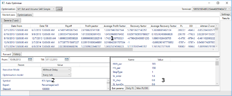
The results tab is also divided into parts, which are marked with numbers to make explanation easier. The first part features optimization passes divided between tabs (Selected pass and Optimisations). The first container tab called "Selected pass" contains selected optimization passes. These passes are divided into two tabs ("Forward" and "History"). Let's see how the optimization parameters are distributed between these tabs. For example, the following dates are specified:

1. 01.01.2012 - 07.12.2012 - History
2. 10.12.2012 - 07.03.2012 - Forward

Optimization will be performed in the historical interval. Then the best parameters will be selected using filtering and sorting (see the description in the previous chapter). Two tests are performed after selection: one on the historical and the other one on the forward interval. Further, testing results of the best parameters are added to the "Selected pass" tab, where they are divided between the "History" and "Forward" tabs. The optimization passes are added to the "Optimisations" tab where you can view the whole list of optimizations for any historical interval. Consider the optimizations tab in more detail.

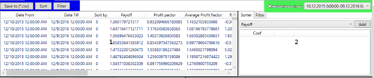
The table structure (the first part of the "Optimisations" tab) is similar to the structure of "Forward" and "History" tabs. But this table shows all optimization passes within the requested interval. The desired time interval can be selected from the "Optimisation dates" combobox. When a new interval is selected, the entire table with the optimization passes is updated. The second part of the tab is similar to the third part of the "Settings" window, and all changes in these tabs are synchronized.

Both the "Optimisations" and the "Selected pass" tabs contain the "Save to (*.csv)" button. When this button is clicked for "Selected pass", a *.csv file is created containing the list of historical and forward optimization passes. When the button is clicked for "Optimisations", information about all performed optimizations is downloaded to the appropriate *csv file. Buttons "Sort" and "Filter" are only available in the "Optimisations" tab. Their purpose is to provide the filtering and sorting of resulting optimization passes in accordance with the settings specified in the second part of the "Optimisations" tab. In practice this option is not required because the auto optimizer uses the same mechanism. However, the option allows using any desired custom filtering. 

Both tables are interactive. A single click on a table row updates the second and third parts of the "Result" tab in accordance with the selected optimization pass. A double-click launches a test in the terminal. In this case, the terminal will not be closed after the end of testing. So you should close it manually after studying the results. Some tester parameters can be configured before starting a test: the second part of the "Results" tab.

  

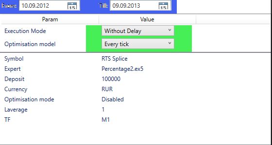
Test start and end dates are updated automatically in accordance with the selected time interval. However, they can be changed by a double click on the desired row. You can also select execution delay and testing type (ticks, OHLC etc.). "No delay" and "Every tick" are set by default. 

The third part of the tab shows the trading statistics for the selected optimization pass (Daily PL and Max PL/DD) and the robot parameters for the selected pass (Bot params tab). The "Max PL/DD" tab does not show the final profit/loss value, but it only shows the total profit (the sum of all profitable deals) and the total loss (the sum of all losing deals). Profit and maximum drawdown registered at the trading completion time are displayed in the table with the optimizations and test result. The Daily PL tab shows the average daily profit and the average daily loss, similarly to the report available in the terminal.

Another simplest algorithm for working with the auto optimizer

Let's consider a ready example of a robot working with the auto optimizer. We already considered the algorithm template in the third article in this series. Now, let's adapt the template for an algorithm in C style. First, we will consider the algorithm itself. It is an algorithm of 2 moving averages. Positions are closed either by a fixed Stop Loss or by a fixed Take Profit. The implementation of functions describing the EA logic are removed from the below code as this is not the purpose of the example.

//+------------------------------------------------------------------+
//|                                                     SimpleMA.mq5 |
//|                        Copyright 2019, MetaQuotes Software Corp. |
//|                                             https://www.mql5.com |
//+------------------------------------------------------------------+
#property copyright "Copyright 2019, MetaQuotes Software Corp."
#property link      "https://www.mql5.com"
#property version   "1.00"

#include <Trade/Trade.mqh>
#define TESTER_ONLY

input int ma_fast = 10; // MA fast
input int ma_slow = 50; // MA slow
input int _sl_ = 20; // SL
input int _tp_ = 60; // TP
input double _lot_ = 1; // Lot size

int ma_fast_handle,ma_slow_handle;
const double tick_size = SymbolInfoDouble(_Symbol,SYMBOL_TRADE_TICK_SIZE);
CTrade trade;

//+------------------------------------------------------------------+
//| Expert initialization function                                   |
//+------------------------------------------------------------------+
int OnInit()
  {
//---

#ifdef TESTER_ONLY
   if(MQLInfoInteger(MQL_TESTER)==0 &&
      MQLInfoInteger(MQL_OPTIMIZATION)==0)
     {
      Print("This expert was created for demonstration! It is not enabled for real trading !");
      ExpertRemove();
      return(INIT_FAILED);
     }
#endif

   ma_fast_handle = iMA(_Symbol,PERIOD_CURRENT,ma_fast,0,MODE_EMA,PRICE_CLOSE);
   ma_slow_handle = iMA(_Symbol,PERIOD_CURRENT,ma_slow,0,MODE_EMA,PRICE_CLOSE);

   if(ma_fast_handle == INVALID_HANDLE ||
      ma_slow_handle == INVALID_HANDLE)
     {
      ExpertRemove();
      return(INIT_FAILED);
     }
//---
   return(INIT_SUCCEEDED);
  }
//+------------------------------------------------------------------+
//| Expert deinitialization function                                 |
//+------------------------------------------------------------------+
void OnDeinit(const int reason)
  {
   if(ma_fast_handle != INVALID_HANDLE)
      IndicatorRelease(ma_fast_handle);
   if(ma_slow_handle != INVALID_HANDLE)
      IndicatorRelease(ma_slow_handle);
  }

enum Direction
  {
   Direction_Long,
   Direction_Short,
   Direction_None
  };

//+------------------------------------------------------------------+
//| Calculate stop                                                   |
//+------------------------------------------------------------------+
double get_sl(const double price, const Direction direction)
  {
   ...
  }

//+------------------------------------------------------------------+
//| Calculate take                                                   |
//+------------------------------------------------------------------+
double get_tp(const double price, const Direction direction)
  {
   ...
  }

//+------------------------------------------------------------------+
//| Open position according to direction                             |
//+------------------------------------------------------------------+
void open_position(const double price,const Direction direction)
  {
   ...
  }

//+------------------------------------------------------------------+
//| Get direction                                                    |
//+------------------------------------------------------------------+
Direction get_direction()
  {
   ...
  }

//+------------------------------------------------------------------+
//| Expert tick function                                             |
//+------------------------------------------------------------------+
void OnTick()
  {
   if(!PositionSelect(_Symbol))
     {
      Direction direction = get_direction();
      if(direction != Direction_None)
         open_position(iClose(_Symbol,PERIOD_CURRENT,0),direction);
     }
  }
//+------------------------------------------------------------------+

This EA code part is basic. It is needed to analyze the changes we need to produce to make the EA available in the auto optimizer. 

Please note that the task did not require an efficient EA, so most probably this robot will be losing. The EA has a restriction to avoid its accidental launch in real trading. To remove the limitation (and to be able to launch it in trading) comment the TESTER_ONLY definition. 

What we do in OnOnit is instantiate moving average indicators. Accordingly, the indicators should be deleted in OnDeinit. The Direction enumeration declared in the code is used for determining the direction. Positions are opened by the CTrade class in the open_position function. The entire logic is described in four code lines, in OnTick callback. Now, let's add connection of the required functionality to the robot.

//+------------------------------------------------------------------+
//|                                                     SimpleMA.mq5 |
//|                        Copyright 2019, MetaQuotes Software Corp. |
//|                                             https://www.mql5.com |
//+------------------------------------------------------------------+
#property copyright "Copyright 2019, MetaQuotes Software Corp."
#property link      "https://www.mql5.com"
#property version   "1.00"

#include <Trade/Trade.mqh>
#include <History manager/AutoLoader.mqh> // Include CAutoUploader
#define TESTER_ONLY

input int ma_fast = 10; // MA fast
input int ma_slow = 50; // MA slow
input int _sl_ = 20; // SL
input int _tp_ = 60; // TP
input double _lot_ = 1; // Lot size

// Comission and price shift (Article 2) 
input double _comission_ = 0; // Comission
input int _shift_ = 0; // Shift

int ma_fast_handle,ma_slow_handle;
const double tick_size = SymbolInfoDouble(_Symbol,SYMBOL_TRADE_TICK_SIZE);
CTrade trade;
CAutoUploader * auto_optimiser; // Pointer to CAutoUploader class (Article 3)
CCCM _comission_manager_; // Comission manager (Article 2)

//+------------------------------------------------------------------+
//| Expert initialization function                                   |
//+------------------------------------------------------------------+
int OnInit()
  {
//---

#ifdef TESTER_ONLY
   if(MQLInfoInteger(MQL_TESTER)==0 &&
      MQLInfoInteger(MQL_OPTIMIZATION)==0)
     {
      Print("This expert was created for demonstration! It is not enabled for real trading !");
      ExpertRemove();
      return(INIT_FAILED);
     }
#endif

   ma_fast_handle = iMA(_Symbol,PERIOD_CURRENT,ma_fast,0,MODE_EMA,PRICE_CLOSE);
   ma_slow_handle = iMA(_Symbol,PERIOD_CURRENT,ma_slow,0,MODE_EMA,PRICE_CLOSE);

   if(ma_fast_handle == INVALID_HANDLE ||
      ma_slow_handle == INVALID_HANDLE)
     {
      ExpertRemove();
      return(INIT_FAILED);
     }

   // Set Commission and shift
   _comission_manager_.add(_Symbol,_comission_,_shift_);

   // Add robot params
   BotParams params[];
   APPEND_BOT_PARAM(ma_fast,params);
   APPEND_BOT_PARAM(ma_slow,params);
   APPEND_BOT_PARAM(_sl_,params);
   APPEND_BOT_PARAM(_tp_,params);
   APPEND_BOT_PARAM(_lot_,params);
   APPEND_BOT_PARAM(_comission_,params);
   APPEND_BOT_PARAM(_shift_,params);

   // Add Instance CAutoUploader class (Article3)
   auto_optimiser = new CAutoUploader(&_comission_manager_,"SimpleMAMutex",params);
//---
   return(INIT_SUCCEEDED);
  }
//+------------------------------------------------------------------+
//| Expert deinitialization function                                 |
//+------------------------------------------------------------------+
void OnDeinit(const int reason)
  {
   if(ma_fast_handle != INVALID_HANDLE)
      IndicatorRelease(ma_fast_handle);
   if(ma_slow_handle != INVALID_HANDLE)
      IndicatorRelease(ma_slow_handle);

   // Delete CAutoUploaderclass (Article 3)
   delete auto_optimiser; 
  }

enum Direction
  {
   Direction_Long,
   Direction_Short,
   Direction_None
  };

//+------------------------------------------------------------------+
//| Calculate stop                                                   |
//+------------------------------------------------------------------+
double get_sl(const double price, const Direction direction)
  {
   ...
  }

//+------------------------------------------------------------------+
//| Calculate take                                                   |
//+------------------------------------------------------------------+
double get_tp(const double price, const Direction direction)
  {
   ...
  }

//+------------------------------------------------------------------+
//| Open position according to direction                             |
//+------------------------------------------------------------------+
void open_position(const double price,const Direction direction)
  {
   ...   
  }

//+------------------------------------------------------------------+
//| Get direction                                                    |
//+------------------------------------------------------------------+
Direction get_direction()
  {
   ...
  }

//+------------------------------------------------------------------+
//| Expert tick function                                             |
//+------------------------------------------------------------------+
void OnTick()
  {
   auto_optimiser.OnTick(); // Save current date (Article 3)

   if(!PositionSelect(_Symbol))
     {
      Direction direction = get_direction();
      if(direction != Direction_None)
         open_position(iClose(_Symbol,PERIOD_CURRENT,0),direction);
     }
  }
//+------------------------------------------------------------------+

All new additions are marked with green. Let's consider them in order of appearance. Firstly, we connect the AutoLoader header file which was described in article 3. This file contains the CAutoUploader class, whose task is to download the accumulated trading history. In the OnInit callback, we add commission to the appropriate CCCM class which was described in article 2. Also, we instantiate the CAutoUploader class after adding EA parameters to it. The CAutoUploader class instance is deleted in the OnDeinit callback, which initializes the call of a destructor in which the trading report is saved to an xml file (Article 1). 

The EA logic is unchanged, with the exception of the OnTick callback, in which the OnTick method of the CAutoUploader class is called. The request enables correct saving of testing start and end dates. The CAutoUploader class only works in the tester and does not perform any actions in real trading. 

Conclusion

The presented article describes the functionality of the created Optimizations Manager. As already mentioned at the beginning of this article, the article should be treated as some an instruction of the resulting application. Technical aspects of the application implementation will be described in further articles. The following is attached to the article:

• The Auto Optimizer project
• The described EA code

To run the auto optimizer program, compile it using Visual Studio IDE. Please note that the MQL5/Include/Libraries directory should contain the "ReportManager.dll" library which was described in the first article. It is also available in the attached Auto Optimizer project (compilation is required).