
MQL5 Wizard Techniques you should know (Part 96): Using Wavelet Thresholding and LSTM Network in a Custom Money Management Class
Introduction
We continue this series on different ideas and trade setups that can be explored and tested thanks to the MQL5 Wizard. In the last article where we looked into money management, in our custom class, we married the Suffix Automation Algorithm with an Autoencoder network. The model we had then could be the suitable tool for traders that like exploiting consolidating markets and where the historical "Price DNA" provides some repetitive patterns. It appeared to thrive in these conditions, provided we had a rhythm. This could then beg the question, what happens when the regime changes. For some traders that test volatile markets such as intraday forex or crypto, repeatable and dependable patterns can be rare. The primary obstacle here often seems that the market is static-erratic with high-frequency noise often disguising as prevalent trends.
For this article, we thus move from pattern recognition to signal processing. Instead of looking out for macro repeatable patterns we now attempt to come up with a surgical tool that is best suited for noisy, momentum-driven environments. We build this tool as a custom money management class that merges the algorithm Wavelet-Thresholding (adopted to de-noise log returns) and a Long Short-Term Memory (LSTM) network. We are sticking to the dual-engine approach of our recent articles as we continue with the theme of introducing more adaptability in scaling position size as we strip away static and lagging signals.
Target Market and Concerns:
Since we now know the last money management article that used the Suffix Automaton was targeted for ranging markets with "historical-echo-patterns", it is worth emphasizing that this Wavelet-LSTM combo is for trending markets especially those characterized with volatility. One can argue that this is particularly meant for the high-volatile arenas - intraday Forex, some momentum driven indices, and restless cryptocurrencies. It can be said that in these settings price does not echo, it erupts. These eruptions do lead us to another maddening problem. The whipsaw. Whenever price violently goes through a key level, how do we establish if it's a genuine trend or market noise? We have posed this question a few times prior in this series however we have not used the Wavelet-LSTM algorithm-network combination as a possible solution, till now.
Sizing positions when the markets are jagged and very uncertain can be very challenging. If one treats every sudden price spike as a valid breakout in volatility, one will over-reduce position size and lead to a tepid performance. And the flip-side of this is worse because mis-reading seemingly moderate price increases as tepid volatility can bleed out an account. So our challenge today therefore will be exploiting another approach at scaling risk, when the real market signal is buried in static.
Model Description
In tackling the whipsaw problem we opt not to depend on just one signal generator or indicator. Rather, as has ben the case so far in these articles, we stick to the dual-engine approach where one "engine" is tasked with aggressively cleaning the data, while the second "engine" is charged with interpreting the surviving sequence from the cleaning.
Engine 1: Wavelet Thresholding (aka the Filter):
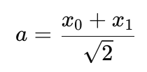
This algorithm can be thought of as a pair of high-end noise-cancelling headphones. These headphones do not alter the underlying music, (which in our case can be understood as price action), but rather they remove the background static so that one can better listen to the bassline (think price trend). Therefore in this case, instead of searching for repeating historical DNA, we process raw chaotic log-returns at the present time. The mathematical definition of this algorithm is set by the discrete Haar Wavelet Transform. This decomposes a sequence of log-returns (x_0, x_1, ..., x_n) into two things, approximation and detail coefficients:
- The approximation coefficients which can represent a trend is set by the formula:
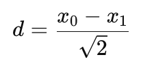
- The detail coefficients which are a proxy for noise is defined by:
Once we have a decomposition, we apply a "soft-thresholding" to the 'detail' coefficients. Whenever the absolute value of a detail coefficient |d| is below a tuned threshold (lambda), we set this coefficient to zero. If it matches or exceeds, we then shrink it as follows:
d = sign(d)(|d| - lambda)
This step quietens high-frequency chatter before we rebuild the signal.
Engine 2: The LSTM Network (The Gatekeeper):
When the Wavelet goes past the static, the Long Short-Term Memory (LSTM) network comes in. So, the Wavelet is meant to clean present data, and the LSTM gives temporal-context or establishes the time connection for the processed data sequence. We also try to address the vanishing gradient problem presented by regular RNNs by using a gated cell. This is meant to manage long-term memory. The main component of our LSTM cell is ruled by the following state update equation:
![]()
Where:
- f_t (Forget Gate): Setting the past information that needs to be discarded with the Sigmoid activation: Sigma(W_f * |h_t-1, x_t| + b_f)
- i_t (Input Gate): Decides which new information to store.
- ~c_t (Candidate State): By using tanh we create a new information candidate.
- c_t (Cell State): This holds the "trend trajectory" as the updated internal memory.
Given that we are pushing the de-noised Wavelet output through these gates, the network then checks for the consistency of the current trend. The output of our calculation is a final confidence coefficient, that serves as a dynamic lot sizing multiplier. This enables the model to recall whether recent volatility was for a valid breakout or a stretch of noise-driven whipsaws. With this feedback we would adjust our exposure accordingly.
MQL5 Implementation
Moving tis dual-engine approach into MQL5 as a custom class for money management implies we have to inherit from the standard 'CExpertMoney' base class. By overriding this base class's virtual functions of 'CheckOpenLong()', and 'CheckOpenShort()' we get to dynamically intercept and scale down or up the volume following any signal generated by the Expert Advisor.
Nonetheless, before we get into the details of this code, we probably need to take on the issue of market sensors. In the last article where we had a custom money management class, we used the Suffix Automaton where we strictly depended on raw price strings since we were setting up for trading price-structure in repeatable/cyclic markets. For our approach in this article, we are looking to tackle volatile/ noisy market environments and therefore raw price analysis is insufficient. We need more context. In order to get this we rely on initializing two native indicators: the Relative Strength Index, and the Average True Range. Why these two?
- RSI (Momentum and Extremes Indicator): When the markets are whipsawing, a sudden price pop could be deemed as a localized anomaly. The RSI oscillator though, can help validate if this move marks sustained momentum of a denoised signal. This is helpful to us in gauging whether a move represents a trend continuation or is an over extended trap.
- ATR (Volatility Benchmark Indicator): Quite often, in order for trader positions to survive volatile markets, they need to have a baseline. The ATR provides us a quantifiable metric of current market displacement. When our Wavelet filter spots a strong signal, we cross-reference it with the ATR in order to validate the volatility breakout. This helps determine how aggressively we would need to down size our positions.
We thus use the RSI, and ATR as extra checks and metrics in gauging up volatility environments. The model in our class 'CMoneyWaveletLSTM' is now covered below, sequentially, starting with the algorithm, then indicator driven modes, and then the neural network.
Step 1: The Wavelet Filter:
At the core of our noise cancelling engine is the anchor class 'CWaveletThreshold'. This helper class does not iterate through historical data points and arrays when seeking matching patterns, as we did with the Suffix Automaton. This class runs a 1-level Haar Discrete Transform (DWT) on the recent log-returns, the Eurler's Log of the ratios between close prices. Lets start by looking at the 'DeNoiseLogReturns' method within this class, and see how we strip away market static:
   //--- De-noises log-returns and returns the sum of the filtered signal
   double            DeNoiseLogReturns(const double &log_returns[])
     {
      int n = ArraySize(log_returns);
      if(n % 2 != 0)
         n -= 1; // Ensure even length for Haar pairs
The Haar Transform needs pairs of data points in order to work out differences and means. We start by checking the array size 'n'. If the history length given is an odd number we just deduct 1 to keep it at even length. This averts out-of-bounds array errors in the loop iteration.
      double approx[];
      double detail[];
      ArrayResize(approx, n / 2);
      ArrayResize(detail, n / 2);
In the listing above, we declare and size two dynamic arrays. These are named 'approx' and 'detail'. Given that we are compressing pairs of data points into single coefficients, the size of these arrays will be precisely half our history length.
      //--- 1. Decomposition (Haar Transform)
      for(int i = 0; i < n / 2; i++)
        {
         approx[i] = (log_returns[2 * i] + log_returns[2 * i + 1]) / MathSqrt(2.0);
         detail[i] = (log_returns[2 * i] - log_returns[2 * i + 1]) / MathSqrt(2.0);
        }
With these declared we move on to the main decomposition logic of our function. What we are doing above is iterating through the log-returns in steps of two.
- The Approximation Coefficient ('approx') is meant to capture the trend. By averaging the pair and scaling it by (1/Sqrt(2)) in order to preserve energy.
- The Detail Coefficient ('detail') is meant to grab high-frequency noise. It works out the difference between the pair, and also scales by the fraction (1/Sqrt(2)). In a very volatile environment, the whipsaws and static can easily be grabbed entirely within this detail array.
      //--- 2. Soft Thresholding (De-noising at specific scale)
      for(int i = 0; i < n / 2; i++)
        {
         if(MathAbs(detail[i]) < m_threshold)
            detail[i] = 0.0; // Filter out noise
         else
            detail[i] = (detail[i] > 0) ? (detail[i] - m_threshold) : (detail[i] + m_threshold);
        }
In the subsequent listing above, is where the noise cancellation takes place. We apply a soft thresholding. When looping through the high-frequency 'detail' coefficients, if the absolute magnitude of a detail coefficient is smaller than the user input 'm_threshold', we take that as an indication of meaningless market static. This gets the coefficient value reset to 0.0. However if it is larger, we shrink it toward zero by the threshold amount. The last step prevents jarring or jumps in our final signal and smooths out aggressive spikes that can be a feature of our target volatile markets.
      //--- 3. Reconstruction & Signal Aggregation
      double denoised_sum = 0.0;
      for(int i = 0; i < n / 2; i++)
        {
         double r0 = (approx[i] + detail[i]) / MathSqrt(2.0);
         double r1 = (approx[i] - detail[i]) / MathSqrt(2.0);
         denoised_sum += (r0 + r1);
        }
Our final step in this function is to reconstruct the sequence. Essentially we reverse the Haar math. We combine our preserved 'approx' trend coefficients with the newly filtered or denoised 'detail' coefficients to recreate log-returns ('r0' and 'r1'). These get aggregated into one clean directional signal that is meant to capture the underlying momentum of recent price action. The theory here is that we have now stripped the log returns of high-frequency static.
Step 2: Four Strategy Modes:
Once we have a clean, 'denoised_sum' output, we then need to decide how to respond to its contents. Given that we are targeting volatile markets, a 'one size fits all' approach is bound to be unsuccessful. Therefore, as in recent articles, we introduce the 'm_algo_mode' parameter that can allow us to select the best approach depending on the asset and markets being traded at the time. It allows us to choose from four distinct functions. Every function evaluates the Wavelet Signal against the RSI and ATR inorder to output a lot sizing multiplier.
Mode 1: Momentum & Trend Following:
//+------------------------------------------------------------------+
//| Mode 1: Momentum & Trend Following                               |
//| Relies heavily on Denoised Signal matching RSI trend.            |
//+------------------------------------------------------------------+
double CMoneyWaveletLSTM::Mode1_MomentumTrend(double signal, double rsi, double atr)
  {
//--- Bullish momentum confirmation
   if(signal > 0 && rsi > 55.0)
      return 1.5;
//--- Bearish momentum confirmation
   if(signal < 0 && rsi < 45.0)
      return 1.5;
//--- Choppy/Divergence - reduce lot size
   return 0.7;
  }
This mode is meant for aggressive trend-follower that is riding a breakout. It requires agreement. When the Wavelet 'signal' is positive (bullish) and the RSI confirms we are in an upward move (> 55.0), we would adjust our lot multiplier to 1.5x. The inverse would apply when doing bearish runs. However when the algorithm and indicator do not agree (diverge), the model would assume the market is in a choppy phase and therefore position sizing would be defensively scaled down to a multiplier of 0.7x.
Mode 2: Mean Reversion:
//+------------------------------------------------------------------+
//| Mode 2: Mean Reversion                                           |
//| Fades the denoised signal when RSI reaches extreme bounds.       |
//+------------------------------------------------------------------+
double CMoneyWaveletLSTM::Mode2_MeanReversion(double signal, double rsi, double atr)
  {
//--- Overbought, anticipate reversal
   if(rsi > 70.0 && signal > 0)
      return 1.25;
//--- Oversold, anticipate reversal
   if(rsi < 30.0 && signal < 0)
      return 1.25;
//--- Normal market conditions - cautious allocation
   return 0.8;
  }
Conversely, in mode-2, we target overextended environments where snapbacks happen a lot. We are trying to spot the extremes here and when the RSI is overbought (> 70.0) but the Wavelet is still pushing positive and yet we anticipate an imminent mean-reversion or collapse. With such an outlook, we would bump our sizing to 1.25x in order to capitalize on the fade. Normal or non-extreme conditions would attract a penalty with lot multiplier shrinking to 0.8x.
Mode 3: Volatility Breakout:
//+------------------------------------------------------------------+
//| Mode 3: Volatility Breakout (ATR Driven)                         |
//| Scales position if denoised momentum breaks above recent ATR.    |
//+------------------------------------------------------------------+
double CMoneyWaveletLSTM::Mode3_VolatilityBreakout(double signal, double rsi, double atr)
  {
//--- Transform signal strength context back to price scale roughly
   double pseudo_price_momentum = MathAbs(signal) * 1000.0;
   if(pseudo_price_momentum > atr)
      return 2.0; // Breakout confirmed by Wavelet & ATR, aggressive size
   return 0.5; // Stagnant, minimize exposure
  }
With this mode, we are pure volatility hunting. Given that the Wavelet outputs a sum of log-returns (as very small decimal values), we would multiply the absolute signal by '1000.0' in order to approximate it back to a regular price-scale point system ('pseudo_price_momentum'). After this, we compare this cleaned momentum directly against the 'atr'. If our validated, denoised momentum is more than the mean volatility envelope, we would have confirmed a significant breakout. Thanks to this conformation, with our model, we scale up position size 2.0x. If we are unable to confirm, we would scale back the multiplier to 0.5x.
Mode 4: Risk-Averse Filter:
//+------------------------------------------------------------------+
//| Mode 4: Conservative / Risk-Averse Filter                        |
//| Only permits sizing up if volatility is low and trend is stable. |
//+------------------------------------------------------------------+
double CMoneyWaveletLSTM::Mode4_ConservativeFilter(double signal, double rsi, double atr)
  {
//--- Avoid trading heavily during massive extremes (High ATR, Extreme RSI)
   if(rsi > 80.0 || rsi < 20.0)
      return 0.25;
//--- If trend is gentle and denoised signal is consistent, standard sizing
   if(rsi >= 40.0 && rsi <= 60.0)
      return 1.0;
   return 0.6;
  }
This mode can be taken as the "governor". For traders, who arguably are the majority, their primary concern is capital preservation especially in wild market conditions. This mode therefore actively punishes lot sizing when markets are at extremes. When the RSI is violently overbought or oversold, it crushes to 0.25x. Standard lot sizing of 1.0.x would only be permitted if the market is relatively tepid with RSI range-bound between 40 and 60.
Step 3: The LSTM Network Gate:
When the wavelet algorithm and the selected mode have given us a primary lot multiplier, we can pass this baton onto the neural network. Unlike when we had the Autoencoder in a past article, that looked at static snapshots of data, the LSTM is meant for time-based sequence evaluation. In realizing this, we code a streamlined 1D-Cell forward-pass struct to use MQL5 execution speed.
   //--- Calculates LSTM forward pass, returns coefficient [0.5, 1.5]
   double            Calculate(const double &sequence[])
     {
      double h_prev = 0.0, c_prev = 0.0;
To start off the inference that is handled in the 'Calculate' function we initialize the hidden state ('h_prev') and the cell state ('c_prev') to zero. This cell state serves as the network's long-term memory track.
      for(int t = 0; t < ArraySize(sequence); t++)
        {
         double x = sequence[t];
         //--- Simplified 1D-Cell mapping
         double f = Sigmoid(m_Wf[0] * h_prev + m_Wf[1] * x + m_bf[0]);
         double i = Sigmoid(m_Wi[0] * h_prev + m_Wi[1] * x + m_bi[0]);
         double c_tilde = MathTanh(m_Wc[0] * h_prev + m_Wc[1] * x + m_bc[0]);
By iterating chronologically through the given sequence of log-returns, on every time step 't', we extract the current value 'x'. In addition:
- We work out the 'Forget Gate' ('f') by passing the weights and biases through a Sigmoid Activation. This informs the network what portion of the prior memory should be discarded. Process here is values closer to 0 are forgotten while those closer to 1 are kept.
- We calculate the 'Input Gate' ('i'), that establishes which new information from the current step gets restored.
- We compute the 'Candidate State' ('c_tilde') by using a MathTanh activation. This normalizes new potential memory between -1 and 1.
         double c_t = f * c_prev + i * c_tilde;
         double o_t = Sigmoid(m_Wo[0] * h_prev + m_Wo[1] * x + m_bo[0]);
         h_prev = o_t * MathTanh(c_t);
         c_prev = c_t;
        }
With this last portion, the network updates its internal reality. The new cell state ('c_t') is the sum of the retained old memory ('f x c_prev') and the chosen new memory ('i x c_tilde'). We then workout the 'Output Gate ('o_t')' and this dictates the proportion of this new internal memory that needs to be exposed to the outside. Updating of 'h_prev' and 'c_prev' for the next loop iteration is performed, since the LSTM "learns" the trajectory of the time-series as it loops.
      //--- Map final hidden state to a lot multiplier [0.5, 1.5]
      return 0.5 + (Sigmoid(h_prev) * 1.0);
     }
After processing the entire historical sequence 'h_prev' the final hidden state will contain the network's concluding confidence assessment. This final value will then get pushed through a Sigmoid function (compressing it to the 0 to 1 range) and then scaling it. The scaling ensures the LSTM does output a gating multiplier in the 0.5 to 1.5 range where these limits would represent penalty for low confidence on the 0.5 end and a reward for high confidence on the 1.5 end.
Step 4: Main Engine ('Optimize'):
The Optimize function serves as the grand orchestrator for our algorithm and neural network. It is called whenever the Expert Advisor requests to open a Long or Short position and it runs in the chronological sequence necessary to scale our volume up or down.
double CMoneyWaveletLSTM::Optimize(double lots)
  {
   double lot = lots;
   double closes[];
   ArraySetAsSeries(closes, true);
We begin by accepting the base 'lots' computed with our risk input settings. Then we prepare a dynamic array 'closes[]' and assign it as a timeseries so that the index 0 represents the most recent bar.
//--- 1. Fetch Prices
   if(CopyClose(m_symbol.Name(), PERIOD_CURRENT, 0, m_history_length + 1, closes) == m_history_length + 1)
     {
      double log_returns[];
      ArrayResize(log_returns, m_history_length);
      //--- 2. Calculate Log Returns
      for(int i = 0; i < m_history_length; i++)
        {
         //--- Log Return: ln(Price_t / Price_t-1)
         log_returns[i] = MathLog(closes[i] / closes[i + 1]);
        }
In our listing above, we fetch historical close prices based on the input parameter 'm_history_length'. We append this with one to work out the initial difference. We then go through the array via a for-loop to fill the 'log_returns[]' by taking the natural logarithm of the current close price divided by the previous close price. Log returns can be hugely superior to raw prices given that they tend to normalize data and can represent a continuous compounding and also allow the wavelet algorithm to evaluate relative percentage displacement instead of absolute price values.
      //--- 3. Apply Wavelet De-noising
      double denoised_signal = m_wavelet.DeNoiseLogReturns(log_returns);
With our raw, chaotic log-returns all set, we forward them to the algorithm engine. The 'DeNoiseLogReturns' function utilizes the Haar Transform, applying a threshold and giving us back a clean summed up 'denoised_signal'.
      //--- 4. Fetch Indicator Data
      double rsi_buffer[1];
      double atr_buffer[1];
      CopyBuffer(m_handle_rsi, 0, 0, 1, rsi_buffer);
      CopyBuffer(m_handle_atr, 0, 0, 1, atr_buffer);
      double current_rsi = rsi_buffer[0];
      double current_atr = atr_buffer[0];
Prior to evaluating the signal, we would have to get some context. For this, we query the current values of our RSI and ATR indicators and subsequently pull the immediate '[0]' data which would represent the current market state.
      //--- 5. Apply Selected Algorithm Iteration Mode
      double scale_factor = 1.0;
      switch(m_algo_mode)
        {
         case 1:
            scale_factor = Mode1_MomentumTrend(denoised_signal, current_rsi, current_atr);
            break;
         case 2:
            scale_factor = Mode2_MeanReversion(denoised_signal, current_rsi, current_atr);
            break;
         case 3:
            scale_factor = Mode3_VolatilityBreakout(denoised_signal, current_rsi, current_atr);
            break;
         case 4:
            scale_factor = Mode4_ConservativeFilter(denoised_signal, current_rsi, current_atr);
            break;
        }
      lot = lot * scale_factor;
The switch statement routes our logic by basing on the user's chosen 'm_algo_mode'. The mode that is chosen evaluates the trio of variables (denoised signal, RSI, and ATR) and returns the algorithm's lot multiplier as 'scale_factor'. We apply this to our base 'lot'. When a user assigns 'm_use_lstm' as false this is where the dynamic lot sizing ends.
      //--- 6. Gated Mode: Apply the LSTM Network
      if(m_use_lstm)
        {
         //--- Normalize log returns for network input
         double network_input[];
         ArrayResize(network_input, m_history_length);
         for(int i = 0; i < m_history_length; i++)
            network_input[i] = log_returns[i] * 100.0; // Scaled up
         double lstm_coef = m_lstm.Calculate(network_input);
         lot = lot * lstm_coef;
        }
     }
However, when the LSTM gate is active, we would move onto one more evaluation by the network. Neural networks usually struggle with small numbers therefore we create a 'network_input[]' array that goes through the 'log_returns', multiplying each by '100.0' to scale them up to a healthy range usable by activation functions. This time-series is fed into the function 'm_lstm.Calculate()'. The network evaluates the sequence, recalls the trajectory and returns its 'lstm_coef' which should be between 0.5 and 1.5. We then multiply our target volume one final time with the multiplier to get the ideal position sizing.
//--- 7. Broker limits validation
   double stepvol = m_symbol.LotsStep();
   lot = stepvol * NormalizeDouble(lot / stepvol, 0);
   double minvol = m_symbol.LotsMin();
   if(lot < minvol)
      lot = minvol;
   double maxvol = m_symbol.LotsMax();
   if(lot > maxvol)
      lot = maxvol;
   return NormalizeDouble(lot, 2);
  }
These concluding lines are standard. Essentially MQL5 money management sanitation. Regardless of the multipliers our dual engine mode produced, we need to conform to the strict operational limits of the broker being traded with. We normalize this lot size to ensure its in line with the symbol's 'LotStep()' requirements and also strictly clamp the volume between the broker's defined 'LotsMin()' and 'LotsMax()' limits. This has to be done before the final volume amount is returned to the Expert Advisor.
Post-Optimization Analysis
To better appreciate the practical impact of this dual-engine model we, as even in the last articles, ran two optimizations. The first observed the Wavelet filter solo while the second was the fully gated model that included the Wavelet and the LSTM. We were testing with the forex pair USD JPY on the 2-hour timeframe from 2025.01.01 to 2026.05.01. As always the forward walk period was 2026 with 2025 being the optimization period. We are testing with the built-in entry signals of Envelopes and RSI.
Run 1: Standalone Wavelet:
In the first optimization and subsequent forward walk we disabled the neural network and the optimizer adapted this un-gated setup by choosing a very reactive 'Signal_ThresholdOpen' value of only 20. Since we had no LSTM to evaluate time-series context, the standalone Wavelet filter was trigger-happy. It jumped at almost any smoothed momentum pulse.

The take profit level at 146 points is very subjective to volatile vs calm markets however it does show some promise. Nonetheless the over dependence on signal clarity leaves it vulnerable to steep drawdowns and many false signals as the report indicates.
Run 2: Both Engines:
For the second test we engaged the LSTM gatekeeper and were able to get the following results:

Conclusion
To wrap things here, we revert to where we began. The Suffix Automaton and Autoencoder models from the last article were historians. They were good at spotting repetition and capitalizing on it. However, news-heavy, and volatile market environments do clearly call for different tools if one is to participate in their regime. This is why we have developed and tested the 'CMoneyWaveletLSTM' class above. For traders that are into volatile assets and aggressive trend following, they would not be reliant on historical matches but on a highly specialized fidelity filter. True money management is never a static percentage. By matching your specific market environment with the correct algorithmic and neural tools, your risk exposure becomes a dynamic reflection of the market's immediate clarity.
| name | description |
|---|---|
| wz_96.mq5 | Wizard Assembled Expert Advisor |
| MoneyWaveLetLSTM.mqh | Custom Money Management Class needed in Wizard Assembly |
| r1.set | Input settings for first test run |
| r2.set | Input settings for second test run |
Warning: All rights to these materials are reserved by MetaQuotes Ltd. Copying or reprinting of these materials in whole or in part is prohibited.
This article was written by a user of the site and reflects their personal views. MetaQuotes Ltd is not responsible for the accuracy of the information presented, nor for any consequences resulting from the use of the solutions, strategies or recommendations described.
- Free trading apps
- Over 8,000 signals for copying
- Economic news for exploring financial markets
You agree to website policy and terms of use