Integrating MQL5 with Data Processing Packages (Part 8): Using Graph Neural Networks for Liquidity Zone Recognition

Table of contents:

1. Introduction
2. Model and System Overview
3. Getting Historical Data
4. Getting Started
5. Putting it all Together on MQL5
6. Back Test
7. Conclusion

Introduction

One of the persistent challenges traders face is identifying liquidity zones before price reacts to them. In numerous instances, liquidity pools such as clusters of stop orders around swing highs, swing lows, or consolidation ranges are only recognized after the market has already moved. Traditional indicators often analyze price in a strictly sequential manner—treating each bar independently—without capturing the deeper structural relationships between different price points in the market. For systematic traders building algorithmic strategies, this limitation makes it difficult to programmatically detect how liquidity forms around structural levels, leading to delayed entries, missed opportunities, or trades taken after liquidity has already been consumed.

To address this limitation, we can represent market structure as a graph, where swing highs, swing lows, and structural turning points become nodes, while the relationships between them form edges that describe how price moves through the market. By applying Graph Neural Networks (GNNs) to this structure, the model can learn patterns of interaction between these nodes, allowing it to recognize where liquidity is likely to accumulate or be targeted next. Integrating this approach with MQL5 enables traders to combine advanced data processing and machine learning techniques with automated trading systems, opening the door to smarter liquidity zone recognition and more informed algorithmic decision-making.

Model and System Overview

The model and the Expert Advisor (EA) work together by dividing responsibilities between data preparation, machine learning inference, and trade execution. The EA operates as the real-time market interface inside MetaTrader 5, continuously collecting price data such as highs, lows, closes, and tick volumes. From this data, the EA constructs a structural representation of the market by detecting swing highs and swing lows, which are then organized into a graph where each swing point becomes a node and their structural relationships form edges. These nodes are enriched with features such as price level, swing type, and relative distance to neighboring swings. The prepared node features and edge connections are then passed to the trained Graph Neural Network (GNN) model, which processes the graph and returns predictions indicating the probability or strength of liquidity presence around each structural level.

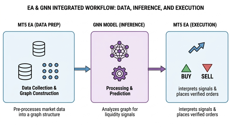
Once the model completes its inference, the EA interprets the returned predictions to determine actionable trading signals. If the model identifies a high probability of liquidity resting above the current market structure, the system may anticipate a bullish move and prepare a buy position, whereas predicted liquidity below the structure may signal a potential sell opportunity. The EA then applies basic trade management rules—such as verifying spread conditions, confirming structural alignment, and calculating position parameters—before executing the order. Through this workflow, the machine learning model focuses on recognizing complex liquidity patterns, while the EA handles the operational aspects of trading, allowing the system to transform graph-based liquidity predictions into automated buy or sell executions within the trading platform.

Getting Historical Data

from datetime import datetime
import MetaTrader5 as mt5
import pandas as pd
import pytz

# Display MetaTrader5 package information
print("MetaTrader5 package author:", mt5.__author__)
print("MetaTrader5 package version:", mt5.__version__)

# Pandas display settings
pd.set_option('display.max_columns', 500)
pd.set_option('display.width', 1500)

# Initialize MT5 connection
if not mt5.initialize():
    print("initialize() failed, error code =", mt5.last_error())
    quit()

# Define symbol
symbol = "XAUUSD.m"

# Ensure the symbol is available
if not mt5.symbol_select(symbol, True):
    print("Failed to select symbol:", symbol)
    mt5.shutdown()
    quit()

# Set timezone to UTC
timezone = pytz.timezone("Etc/UTC")

# Define date range
utc_from = datetime(2025, 11, 1, tzinfo=timezone)
utc_to   = datetime(2026, 2, 28, tzinfo=timezone)

# Get historical rates
rates = mt5.copy_rates_range(symbol, mt5.TIMEFRAME_H1, utc_from, utc_to)

# Shutdown MT5 connection
mt5.shutdown()

# Validate data
if rates is None or len(rates) == 0:
    print("No data retrieved. Check symbol or date range.")
else:
    
    print("First 10 bars:")
    for rate in rates[:10]:
        print(rate)

    # Convert to DataFrame
    rates_frame = pd.DataFrame(rates)

    # Convert time
    rates_frame['time'] = pd.to_datetime(rates_frame['time'], unit='s')

    # Save to CSV
    filename = "XAUUSD_H1.csv"
    rates_frame.to_csv(filename, index=False)

    print("\nData saved to:", filename)

Output:

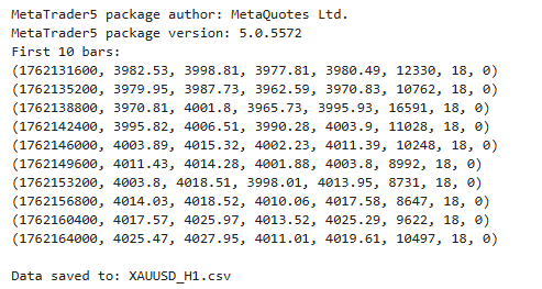
This script establishes a connection between Python and the MetaTrader 5 terminal to retrieve historical market data for analysis and model training. It begins by importing the necessary libraries, displaying the MetaTrader 5 package information, and configuring Pandas display settings for clearer data inspection. After initializing the MetaTrader 5 connection, the script selects the XAUUSD.m symbol and defines a specific historical date range using UTC time. It then requests hourly price data within this period using the copy_rates_range function, which returns structured information such as open, high, low, close, and tick volume.

Getting Started

import pandas as pd
import numpy as np
import torch
import torch.nn.functional as F

from torch_geometric.data import Data
from torch_geometric.nn import GCNConv

from sklearn.preprocessing import StandardScaler

df = pd.read_csv("XAUUSD_H1.csv")
df['time'] = pd.to_datetime(df['time'])
df.head()

Output:

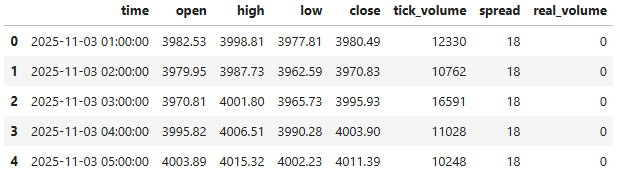
To get started, we import the necessary libraries required for data handling, numerical processing, and building our Graph Neural Network model. We then load the historical XAUUSD H1 dataset from the CSV file we previously generated and convert the time column into a proper datetime format for easier time-based analysis. Finally, we preview the first few rows of the dataset to verify that the data has been loaded correctly and is ready for further preprocessing.

def detect_swings(df, window=3):

    swing_highs = []
    swing_lows = []

    for i in range(window, len(df)-window):

        high = df['high'][i]
        low = df['low'][i]

        if high == max(df['high'][i-window:i+window]):
            swing_highs.append(i)

        if low == min(df['low'][i-window:i+window]):
            swing_lows.append(i)

    return swing_highs, swing_lows

highs, lows = detect_swings(df)

nodes = []
node_prices = []

for i in highs:

    price = df['close'][i]
    volume = df['tick_volume'][i]

    nodes.append([price, volume, 1])
    node_prices.append(price)

for i in lows:

    price = df['close'][i]
    volume = df['tick_volume'][i]

    nodes.append([price, volume, -1])
    node_prices.append(price)

nodes = np.array(nodes)
node_prices = np.array(node_prices)

In this section, we define a function called detect_swings, which is responsible for identifying swing highs and swing lows within the price data. The function scans through the dataset using a specified window size, comparing each candle’s high and low values to the surrounding candles. If a candle’s high is the maximum within the defined range, it is classified as a swing high, while if its low is the minimum within that same range, it is identified as a swing low. The indices of these detected swings are then stored in separate lists, allowing us to locate important turning points in the market structure.

After identifying the swing points, we construct the graph nodes that will later be used by the Graph Neural Network. For each detected swing high and swing low, we extract relevant features such as the closing price and tick volume from the dataset. These values are combined with a structural label—1 for swing highs and -1 for swing lows—to describe the type of market structure represented by each node. All node features are then collected into a NumPy array, while the corresponding price levels are stored separately, preparing the data for the next stage, where the graph structure will be built and processed by the model.

scaler = StandardScaler()
nodes = scaler.fit_transform(nodes)
edges = []

for i in range(len(nodes)-1):

    edges.append([i, i+1])
    edges.append([i+1, i])

edge_index = torch.tensor(edges, dtype=torch.long).t().contiguous()

labels = []

for i in range(len(node_prices)):

    price = node_prices[i]

    # count nearby swing prices
    touches = np.sum(np.abs(node_prices - price) < 1.0)

    if touches >= 3:
        labels.append(1)
    else:
        labels.append(0)

labels = torch.tensor(labels)

unique, counts = np.unique(labels.numpy(), return_counts=True)

print(dict(zip(unique, counts)))

Output:

{np.int64(0): np.int64(311), np.int64(1): np.int64(103)}

Here, we prepare the data so that it can be processed by the Graph Neural Network. We begin by using StandardScaler to normalize the node features, ensuring that values such as price and volume are scaled consistently for more stable model training. Next, we construct the graph edges by connecting each node to its neighboring node in both directions, forming a simple structural graph that represents the sequence of swing points in the market.

We then generate labels for each node by measuring how many other swing prices occur near the same price level; if a price level is touched multiple times within a small range, it is labeled as a potential liquidity zone; otherwise, it is labeled as a normal level. Finally, these labels are converted into tensors, and their distribution is printed, allowing us to quickly verify the balance between liquidity and non-liquidity nodes before training the model.

x = torch.tensor(nodes, dtype=torch.float)

data = Data(
    x=x,
    edge_index=edge_index,
    y=labels
)

print(data)

Output:

Data(x=[414, 3], edge_index=[2, 826], y=[414])

In this step, we convert the processed node feature data into a PyTorch tensor, which allows it to be used by the Graph Neural Network. We then construct a graph data object using the data structure from PyTorch Geometric, combining the node features, edge connections, and target labels into a single graph representation. Finally, we print the graph object to verify that the dataset has been correctly structured and is ready for model training.

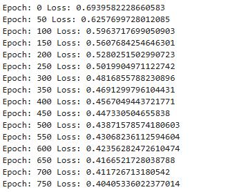
class LiquidityGNN(torch.nn.Module):

    def __init__(self):

        super().__init__()

        self.conv1 = GCNConv(3, 32)
        self.conv2 = GCNConv(32, 32)
        self.conv3 = GCNConv(32, 2)

    def forward(self, x, edge_index):

        x = self.conv1(x, edge_index)
        x = F.relu(x)

        x = self.conv2(x, edge_index)
        x = F.relu(x)

        x = self.conv3(x, edge_index)

        return x

model = LiquidityGNN()

optimizer = torch.optim.Adam(model.parameters(), lr=0.005)

weights = torch.tensor([1.0, 3.0])  # give liquidity higher importance

loss_fn = torch.nn.CrossEntropyLoss(weight=weights)

for epoch in range(800):

    model.train()
    optimizer.zero_grad()
    out = model(data.x, data.edge_index)
    loss = loss_fn(out, data.y)
    loss.backward()
    optimizer.step()

    if epoch % 50 == 0:
        print("Epoch:", epoch, "Loss:", loss.item())

Output:

In this section, we define the LiquidityGNN model, which is a Graph Neural Network designed to analyze relationships between swing points in the market. The model is built using three Graph Convolutional Network (GCN) layers, where the first layer transforms the input node features into a larger feature space, the second layer refines the learned structural information, and the final layer produces output predictions for each node. During the forward pass, the graph convolution operations use both the node features and the edge connections to propagate information between neighboring nodes, while the ReLU activation function introduces non-linearity, allowing the network to learn more complex structural patterns associated with liquidity zones.

After defining the model, we prepare it for training by creating an Adam optimizer and a cross-entropy loss function with weighted classes, giving higher importance to liquidity nodes so the model learns to prioritize them. The training loop then runs for multiple epochs, where the model repeatedly processes the graph data, calculates the prediction loss compared to the true labels, and updates its parameters through backpropagation. Every few iterations, the training loss is printed to monitor the model’s learning progress and ensure that it is gradually improving its ability to identify potential liquidity zones within the graph structure.

model.eval()

pred = model(data.x, data.edge_index).argmax(dim=1)

print(pred)

Output:

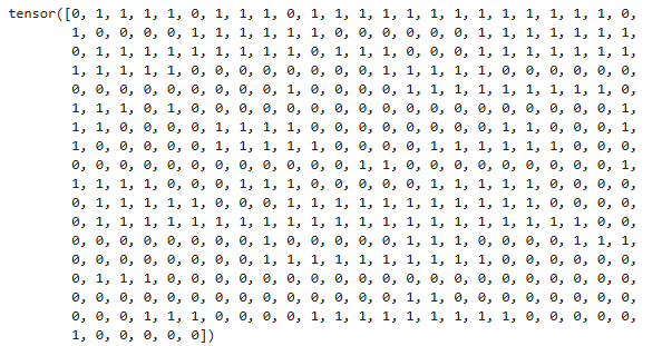
We switch the LiquidityGNN model to evaluation mode to disable training-specific behaviors, then generate predictions for each node by selecting the class with the highest output probability. Then, we print these predicted labels, showing which nodes the model identifies as potential liquidity zones.

liquidity_nodes = (pred == 1).nonzero(as_tuple=True)[0]

print("Liquidity nodes:", liquidity_nodes)

Output:

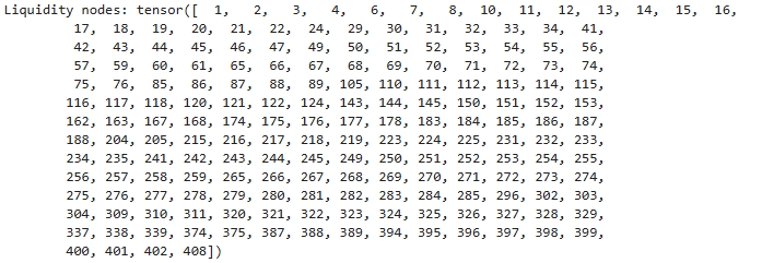
Here, we set the model to evaluate mode and output the predicted class for each node, indicating potential liquidity zones.

import os

mt5_path = r"C:\Users\...\AppData\Roaming\MetaQuotes\Terminal\...\MQL5\Files"

model_path = os.path.join(mt5_path, "liquidity_gnn.onnx")

dummy_x = data.x
dummy_edge = data.edge_index
model.eval()

torch.onnx.export(
    model,
    (dummy_x, dummy_edge),
    model_path,
    input_names=["node_features","edge_index"],
    output_names=["output"],
    opset_version=17,
    do_constant_folding=True,
    external_data=False,
    dynamic_axes={
        "node_features":{0:"nodes"},
        "edge_index":{1:"edges"},
        "output":{0:"nodes"}
    }
)
print("Model saved to:", model_path)

Output:

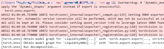
We define the path to MetaTrader 5’s Files directory and specify the ONNX model file location, then set the trained GNN model to evaluation mode and export it to ONNX format using torch.onnx.export, including dynamic axes for nodes and edges to handle varying graph sizes, and finally confirm the model has been saved to the specified path.

Putting it all Together on MQL5

//+------------------------------------------------------------------+
//|                                                     Graph NN.mq5 |
//|                        GIT under Copyright 2025, MetaQuotes Ltd. |
//|                     https://www.mql5.com/en/users/johnhlomohang/ |
//+------------------------------------------------------------------+
#property copyright "GIT under Copyright 2025, MetaQuotes Ltd."
#property link      "https://www.mql5.com/en/users/johnhlomohang/"
#property version   "1.00"
#property strict

#resource "\\Files\\liquidity_gnn.onnx" as uchar ExtModel[]

#include <Trade/Trade.mqh>
#include <ONNXRuntime/ONNXRuntime.mqh>

//--- trading
CTrade trade;

//+------------------------------------------------------------------+
//| Inputs                                                           |
//+------------------------------------------------------------------+
input          string            ModelFile="liquidity_gnn.onnx";
input          int               SwingWindow=3;
input          int               BarsToProcess=500;
input          int               MaxNodes=50;
input          int               MaxEdges=100;
input          double            MinLiquidityScore=0.7;
input          double            LotSize=0.1;
input          int               MagicNumber=777;
input          bool              UseStopLoss=true;
input          int               StopLossPoints=200;
input          bool              UseTakeProfit=true;
input          int               TakeProfitPoints=400;

//+------------------------------------------------------------------+
//| Global variables                                                 |
//+------------------------------------------------------------------+

double               node_features[];
long                 edge_index[];
double               predictions[];
double               nodePrices[];
int                  swingHighs[];
int                  swingLows[];
int                  nodeCount=0;
int                  actualEdgeCount=0;
datetime             lastBarTime=0;
//--- scaler values
double               scalerMean[3]= {1950,500,0};
double               scalerStd[3]= {100,200,1};
long                 onnx_handle;
//--- Model dimensions from ONNX
long                 model_nodes = 0;
long                 model_features = 0;
long                 model_edges = 0;
long                 model_classes = 0;

In this code section, we first embed the trained ONNX GNN model as a resource using #resource, which allows the Expert Advisor to access it directly from the Files folder without relying on external file paths. We then include the necessary MQL5 libraries for trading (CTrade) and ONNX runtime functionality, and define input parameters that control key aspects of the system, such as the swing detection window, number of bars to process, maximum nodes and edges for the graph, minimum liquidity score for trade execution, position sizing, stop-loss/take-profit settings, and a unique MagicNumber to identify trades.

We also declare global variables to hold graph data structures and model outputs, including arrays for node features, edge indices, predictions, and node prices, as well as swing highs and lows. Additional globals track the current number of nodes, actual edges, and the timestamp of the last processed bar. To normalize the data, precomputed mean and standard deviation values are stored in arrays (scalerMean and scalerStd), and placeholders for ONNX model dimensions (nodes, features, edges, classes) and the ONNX session handle are initialized, ensuring the EA is ready to load the model, process incoming price data, and make trade decisions.

//+------------------------------------------------------------------+
//| Expert initialization                                            |
//+------------------------------------------------------------------+
int OnInit()
  {
   trade.SetExpertMagicNumber(MagicNumber);

   onnx_handle = OnnxCreateFromBuffer(ExtModel, ONNX_DEFAULT);

   if(onnx_handle == INVALID_HANDLE)
     {
      Print("ONNX create failed: ", GetLastError());
      return INIT_FAILED;
     }

   Print("ONNX model loaded");

   OnnxTypeInfo type_info;

   long input_count = OnnxGetInputCount(onnx_handle);
   Print("Model inputs: ", input_count);

   for(long i = 0; i < input_count; i++)
     {
      string name = OnnxGetInputName(onnx_handle, i);
      Print("Input ", i, " name: ", name);

      if(OnnxGetInputTypeInfo(onnx_handle, i, type_info))
        {
         Print("Input ", i, " dimensions:");
         ArrayPrint(type_info.tensor.dimensions);

         //--- Store model dimensions
         if(name == "node_features")
           {
            if(ArraySize(type_info.tensor.dimensions) >= 2)
              {
               model_nodes = type_info.tensor.dimensions[0];
               model_features = type_info.tensor.dimensions[1];
               Print("Model expects node_features: [", model_nodes, ", ", model_features, "]");
              }
           }
         else
            if(name == "edge_index")
              {
               if(ArraySize(type_info.tensor.dimensions) >= 2)
                 {
                  model_edges = type_info.tensor.dimensions[1];
                  Print("Model expects edge_index: [2, ", model_edges, "]");
                 }
              }
        }
     }

   long output_count = OnnxGetOutputCount(onnx_handle);
   Print("Model outputs: ", output_count);

   for(long i = 0; i < output_count; i++)
     {
      string name = OnnxGetOutputName(onnx_handle, i);
      Print("Output ", i, " name: ", name);

      if(OnnxGetOutputTypeInfo(onnx_handle, i, type_info))
        {
         Print("Output ", i, " dimensions:");
         ArrayPrint(type_info.tensor.dimensions);

         if(ArraySize(type_info.tensor.dimensions) >= 2)
           {
            model_classes = type_info.tensor.dimensions[1];
            Print("Model output classes: ", model_classes);
           }
        }
     }

//--- Don't set fixed shapes - the model has dynamic axes
//--- Instead, we'll use the actual node count from detection

   Print("ONNX initialization complete");
   Print("Model expects: nodes=", model_nodes, ", features=", model_features,
         ", edges=", model_edges, ", classes=", model_classes);

   return INIT_SUCCEEDED;
  }

//+------------------------------------------------------------------+
//| Expert deinitialization function                                 |
//+------------------------------------------------------------------+
void OnDeinit(const int reason)
  {
   Print("EA deinitializing. Reason code: ", reason);

//--- Release ONNX model session
   if(onnx_handle != INVALID_HANDLE)
     {
      OnnxRelease(onnx_handle);
      onnx_handle = INVALID_HANDLE;
      Print("ONNX session released");
     }

//--- Delete all objects created by this EA
//--- Delete liquidity objects on the chart
   int deleted = 0;
   for(int i = ObjectsTotal(0, -1, OBJ_RECTANGLE) - 1; i >= 0; i--)
     {
      string name = ObjectName(0, i);
      if(StringFind(name, "Liq_") == 0) // Objects starting with "Liq_"
        {
         ObjectDelete(0, name);
         deleted++;
        }
     }

   if(deleted > 0)
      Print("Deleted ", deleted, " rectangle objects");

//--- Optionally close all open positions (if you want this behavior)
   bool closePositions = false; // Set to true if you want to close all positions on deinit

   if(closePositions)
     {
      int closed = 0;
      for(int i = PositionsTotal() - 1; i >= 0; i--)
        {
         ulong ticket = PositionGetTicket(i);
         if(PositionSelectByTicket(ticket))
           {
            if(PositionGetInteger(POSITION_MAGIC) == MagicNumber)
              {
               trade.PositionClose(ticket);
               closed++;
              }
           }
        }

      if(closed > 0)
         Print("Closed ", closed, " positions");
     }

//--- Clear global arrays to free memory
   ArrayFree(node_features);
   ArrayFree(edge_index);
   ArrayFree(predictions);
   ArrayFree(nodePrices);
   ArrayFree(swingHighs);
   ArrayFree(swingLows);

   Print("EA deinitialization complete");
  }

In the OnInit() function, we initialize the Expert Advisor by first assigning the magic number to the CTrade object, ensuring that trades opened by this EA are uniquely identified. We then load the embedded ONNX model from the ExtModel uchar array using OnnxCreateFromBuffer, and check for successful creation. Once the model session is active, we query its input and output specifications using OnnxGetInputCount, OnnxGetInputName, OnnxGetInputTypeInfo, and similar output functions. This allows us to dynamically store the expected number of nodes, features, edges, and output classes, which the EA will later use to correctly format the graph data for inference.

The OnDeinit() function ensures clean shutdown and resource management when the EA is removed or the terminal exits. It first releases the ONNX session to free memory, then iterates through all chart objects to remove any liquidity objects created by the EA. Optionally, it can close all open positions linked to the EA’s magic number. Finally, it clears global arrays used for node features, edge indices, predictions, prices, and swings to free memory.

//+------------------------------------------------------------------+
//| Expert tick                                                      |
//+------------------------------------------------------------------+
void OnTick()
  {
   datetime currentBar = iTime(_Symbol, _Period, 0);

   if(currentBar == lastBarTime)
      return;

   lastBarTime = currentBar;

   if(!DetectSwings())
      return;

   if(!BuildGraph())
      return;

   if(!RunInference())
      return;

   ExecuteTrades();
  }

//+------------------------------------------------------------------+
//| Detect swing highs/lows                                          |
//+------------------------------------------------------------------+
bool DetectSwings()
  {
   ArrayResize(swingHighs, 0);
   ArrayResize(swingLows, 0);

   double high[], low[];

   ArraySetAsSeries(high, true);
   ArraySetAsSeries(low, true);

   if(CopyHigh(_Symbol, _Period, 0, BarsToProcess, high) <= 0)
     {
      Print("Failed to copy high data");
      return false;
     }

   if(CopyLow(_Symbol, _Period, 0, BarsToProcess, low) <= 0)
     {
      Print("Failed to copy low data");
      return false;
     }

   for(int i = SwingWindow; i < BarsToProcess - SwingWindow; i++)
     {
      bool swingHigh = true;
      bool swingLow = true;

      for(int j = -SwingWindow; j <= SwingWindow; j++)
        {
         if(j == 0)
            continue;

         if(high[i] <= high[i + j])
            swingHigh = false;

         if(low[i] >= low[i + j])
            swingLow = false;
        }

      if(swingHigh)
        {
         int s = ArraySize(swingHighs);
         ArrayResize(swingHighs, s + 1);
         swingHighs[s] = i;
        }

      if(swingLow)
        {
         int s = ArraySize(swingLows);
         ArrayResize(swingLows, s + 1);
         swingLows[s] = i;
        }
     }

   Print("Detected ", ArraySize(swingHighs), " swing highs and ",
         ArraySize(swingLows), " swing lows");

   return true;
  }

In the OnTick() function, we handle the core logic of the EA on every incoming tick. The function first checks if a new bar has formed by comparing the timestamp of the current bar with lastBarTime; if it hasn’t, the function exits early to avoid redundant calculations. Once a new bar is detected, the EA sequentially calls DetectSwings() to identify recent swing highs and lows, BuildGraph() to create the graph representation for the ONNX model, RunInference() to obtain liquidity predictions from the GNN, and finally ExecuteTrades() to place buy or sell orders based on the predicted signals.

The DetectSwings() function scans recent bars to identify local maxima and minima, representing swing highs and lows. Using a configurable SwingWindow, it iterates through the high and low price arrays and compares each bar against its surrounding neighbors to determine if it qualifies as a swing. Detected swings are stored in dynamic arrays swingHighs and swingLows. The function also handles errors in copying price data and prints out a summary of the number of swings detected, providing transparency and debugging insight. This step is crucial as it forms the foundational nodes for building the graph that the GNN uses for liquidity analysis.

//+------------------------------------------------------------------+
//| Build graph                                                      |
//+------------------------------------------------------------------+
bool BuildGraph()
  {
   double close[];
   long volume[];

   ArraySetAsSeries(close, true);
   ArraySetAsSeries(volume, true);

   if(CopyClose(_Symbol, _Period, 0, BarsToProcess, close) <= 0)
     {
      Print("Failed to copy close data");
      return false;
     }

   if(CopyTickVolume(_Symbol, _Period, 0, BarsToProcess, volume) <= 0)
     {
      Print("Failed to copy volume data");
      return false;
     }

   nodeCount = 0;
   ArrayResize(nodePrices, MaxNodes);

//--- swing highs
   for(int i = 0; i < ArraySize(swingHighs) && nodeCount < MaxNodes; i++)
     {
      int bar = swingHighs[i];
      if(bar < BarsToProcess)
        {
         nodePrices[nodeCount] = close[bar];
         nodeCount++;
        }
     }

//--- swing lows
   for(int i = 0; i < ArraySize(swingLows) && nodeCount < MaxNodes; i++)
     {
      int bar = swingLows[i];
      if(bar < BarsToProcess)
        {
         nodePrices[nodeCount] = close[bar];
         nodeCount++;
        }
     }

   if(nodeCount < 2)
     {
      Print("Not enough nodes: ", nodeCount);
      return false;
     }

   Print("Building graph with ", nodeCount, " nodes");

//--- Build node features [nodes, 3]
   ArrayResize(node_features, nodeCount * 3);
   ArrayInitialize(node_features, 0);

   int f = 0;
   for(int i = 0; i < nodeCount; i++)
     {
      double price = nodePrices[i];
      double vol = 0;

      //--- Get volume for this bar
      if(i < BarsToProcess)
         vol = (double)volume[i];

      //--- Determine swing type (1 for highs, -1 for lows)
      double swingType = (i < ArraySize(swingHighs)) ? 1.0 : -1.0;

      //--- Normalize features using scaler
      node_features[f++] = (price - scalerMean[0]) / scalerStd[0];  // price
      node_features[f++] = (vol - scalerMean[1]) / scalerStd[1];    // volume
      node_features[f++] = (swingType - scalerMean[2]) / scalerStd[2]; // swing type
     }

//--- Build edges
//--- For a chain graph with bidirectional connections between consecutive nodes:
//--- Number of edges = (nodeCount - 1) * 2
   actualEdgeCount = (nodeCount - 1) * 2;

//--- Edge_index should be a flattened array of shape [2, actualEdgeCount]
//--- That means: [row0_edge0, row1_edge0, row0_edge1, row1_edge1, ...]
//--- So total array size = 2 * actualEdgeCount
   int edgeArraySize = 2 * actualEdgeCount;
   ArrayResize(edge_index, edgeArraySize);
   ArrayInitialize(edge_index, 0);

   Print("Creating ", actualEdgeCount, " edges, array size: ", edgeArraySize);

   int e = 0;
   for(int i = 0; i < nodeCount - 1; i++)
     {
      //--- Forward edge: from i to i+1
      if(e < edgeArraySize - 1)
        {
         edge_index[e] = 0;     // row 0 (source row)
         e++;
         edge_index[e] = i;      // source node index
         e++;
        }

      //--- Forward edge: target
      if(e < edgeArraySize - 1)
        {
         edge_index[e] = 1;      // row 1 (target row)
         e++;
         edge_index[e] = i + 1;  // target node index
         e++;
        }

      //--- Backward edge: from i+1 to i (source)
      if(e < edgeArraySize - 1)
        {
         edge_index[e] = 0;      // row 0 (source row)
         e++;
         edge_index[e] = i + 1;  // source node index
         e++;
        }

      //--- Backward edge: target
      if(e < edgeArraySize - 1)
        {
         edge_index[e] = 1;      // row 1 (target row)
         e++;
         edge_index[e] = i;      // target node index
         e++;
        }
     }

   Print("Added ", e/2, " edge entries (", e, " array elements used)");

//--- Verify we used the correct number of elements
   if(e != edgeArraySize)
     {
      Print("Warning: Expected ", edgeArraySize, " elements but used ", e);
     }

   return true;
  }

//+------------------------------------------------------------------+
//| Run ONNX inference                                               |
//+------------------------------------------------------------------+
bool RunInference()
  {
//--- Set dynamic shapes before inference
   long input0_shape[] = {nodeCount, 3};
   if(!OnnxSetInputShape(onnx_handle, 0, input0_shape))
     {
      Print("Failed to set input shape for node_features: ", GetLastError());
      return false;
     }

//--- actualEdgeCount is the number of edges (not the array size)
//--- Edge_index shape is [2, actualEdgeCount]
   long input1_shape[] = {2, actualEdgeCount};
   if(!OnnxSetInputShape(onnx_handle, 1, input1_shape))
     {
      Print("Failed to set input shape for edge_index: ", GetLastError());
      return false;
     }

   long output_shape[] = {nodeCount, 2};
   if(!OnnxSetOutputShape(onnx_handle, 0, output_shape))
     {
      Print("Failed to set output shape: ", GetLastError());
      return false;
     }

//--- Debug: Print array sizes
   Print("Running inference with: nodes=", nodeCount,
         ", edges=", actualEdgeCount,
         ", features array size=", ArraySize(node_features),
         ", edges array size=", ArraySize(edge_index));

//--- Run inference
   ArrayResize(predictions, nodeCount * 2);

   if(!OnnxRun(onnx_handle, ONNX_NO_CONVERSION, node_features, edge_index, predictions))
     {
      Print("ONNX inference failed: ", GetLastError());
      return false;
     }

   ProcessPredictions();

   return true;
  }

The BuildGraph() function constructs the graph representation of recent market swings that will be fed into the ONNX GNN model. It first gathers the latest close prices and tick volumes for the specified number of bars, then combines the detected swing highs and lows into a node array. Each node is assigned three features—normalized price, volume, and swing type (high=1, low=-1)—using predefined scaler values. The function also builds bidirectional edges between consecutive nodes to form a chain graph, storing them in a flattened edge_index array, while keeping track of the total node and edge counts for dynamic ONNX input sizing.

The RunInference() function then prepares the dynamic input and output shapes based on the actual number of nodes and edges created in BuildGraph(). It resizes the ONNX input tensors (node_features and edge_index) and output tensor, prints debug information for verification, and executes the ONNX model using OnnxRun(). Predictions are stored in the predictions array and processed by ProcessPredictions(). This step directly translates the graph representation of market swings into actionable liquidity signals that the EA can later use to trigger trades, ensuring real-time inference aligns with the dynamically detected market structure.

//+------------------------------------------------------------------+
//| Process predictions                                              |
//+------------------------------------------------------------------+
void ProcessPredictions()
  {
   int liquidityCount = 0;

   for(int i = 0; i < nodeCount; i++)
     {
      double p0 = predictions[i * 2];
      double p1 = predictions[i * 2 + 1];

      //--- Apply softmax manually
      double maxv = MathMax(p0, p1);
      double e0 = MathExp(p0 - maxv);
      double e1 = MathExp(p1 - maxv);
      double prob = e1 / (e0 + e1);  // Probability of class 1 (liquidity)

      if(prob > MinLiquidityScore)
        {
         liquidityCount++;
         DrawLiquidityZone(i, nodePrices[i], prob);
        }
     }

   if(liquidityCount > 0)
      Print("Found ", liquidityCount, " liquidity zones");
  }

//+------------------------------------------------------------------+
//| Execute trades                                                   |
//+------------------------------------------------------------------+
void ExecuteTrades()
  {
   if(CountPositions() > 0)
      return;

   double ask = SymbolInfoDouble(_Symbol, SYMBOL_ASK);
   double bid = SymbolInfoDouble(_Symbol, SYMBOL_BID);

   for(int i = 0; i < nodeCount; i++)
     {
      if(MathAbs(nodePrices[i] - ask) < 10 * _Point)
        {
         if(ask < nodePrices[i])
            OpenTrade(ORDER_TYPE_BUY);
         else
            OpenTrade(ORDER_TYPE_SELL);
         break;
        }
     }
  }

//+------------------------------------------------------------------+
//| Open trade                                                       |
//+------------------------------------------------------------------+
void OpenTrade(ENUM_ORDER_TYPE type)
  {
   double price, sl = 0, tp = 0;

   if(type == ORDER_TYPE_BUY)
      price = SymbolInfoDouble(_Symbol, SYMBOL_ASK);
   else
      price = SymbolInfoDouble(_Symbol, SYMBOL_BID);

   if(UseStopLoss)
     {
      if(type == ORDER_TYPE_BUY)
         sl = price - StopLossPoints * _Point;
      else
         sl = price + StopLossPoints * _Point;
     }

   if(UseTakeProfit)
     {
      if(type == ORDER_TYPE_BUY)
         tp = price + TakeProfitPoints * _Point;
      else
         tp = price - TakeProfitPoints * _Point;
     }

   if(type == ORDER_TYPE_BUY)
      trade.Buy(LotSize, _Symbol, price, sl, tp);
   else
      trade.Sell(LotSize, _Symbol, price, sl, tp);
  }

//+------------------------------------------------------------------+
//| Draw zone                                                        |
//+------------------------------------------------------------------+
void DrawLiquidityZone(int id, double price, double probability)
  {
   string name = "Liq_" + IntegerToString(id) + "_" + IntegerToString(TimeCurrent());

   datetime t1 = iTime(_Symbol, _Period, 0);
   datetime t2 = t1 + PeriodSeconds(_Period) * 5;

   if(!ObjectCreate(0, name, OBJ_RECTANGLE, 0,
                    t1, price - 5 * _Point,
                    t2, price + 5 * _Point))
     {
      Print("Failed to create rectangle object");
      return;
     }

   ObjectSetInteger(0, name, OBJPROP_COLOR, clrGold);
   ObjectSetInteger(0, name, OBJPROP_FILL, true);
   ObjectSetString(0, name, OBJPROP_TEXT, "Liquidity: " + DoubleToString(probability * 100, 1) + "%");
  }

The ProcessPredictions() function takes the raw outputs from the ONNX GNN model and converts them into actionable liquidity probabilities for each detected node. For every node, it manually applies a softmax calculation to determine the likelihood that the node represents a significant liquidity zone. Nodes that exceed the user-defined MinLiquidityScore threshold are counted and visualized on the chart using DrawLiquidityZone(), creating rectangular zones around the predicted price levels with color and probability labels. This allows traders to see where the model identifies potential areas of high liquidity in the market.

The subsequent trading logic leverages these identified liquidity zones to execute positions automatically. ExecuteTrades() first checks that there are no existing open positions and then compares current ask and bid prices to the detected node prices. When the price is within a tight range of a node, the system opens a buy or sell trade accordingly using OpenTrade(), which applies configurable stop-loss and take-profit levels. The DrawLiquidityZone() function ensures each liquidity zone is clearly marked on the chart with a rectangle and annotated probability, providing both visual context and automated execution signals for the EA.

//+------------------------------------------------------------------+
//|                                                  ONNXRuntime.mqh |
//|                        GIT under Copyright 2025, MetaQuotes Ltd. |
//|                     https://www.mql5.com/en/users/johnhlomohang/ |
//+------------------------------------------------------------------+
#property copyright "GIT under Copyright 2025, MetaQuotes Ltd."
#property link      "https://www.mql5.com/en/users/johnhlomohang/"

//--- ONNX flags (keep it in sync with MT5 if changed)
#define ONNX_DEFAULT       0
#define ONNX_DEBUG_LOGS    1
#define ONNX_NO_CONVERSION 2

//--- Simple ONNX model wrapper that calls MT5 built-in Onnx* functions.
//--- This wrapper DOES NOT redeclare OnnxTypeInfo and DOES NOT import any DLL.

//+------------------------------------------------------------------+
//|                     Simple ONNX Runtime Wrapper                  |
//+------------------------------------------------------------------+
class CSimpleONNXModel
  {
private:
   long              session;
   bool              initialized;

public:

                     CSimpleONNXModel()
     {
      session = INVALID_HANDLE;
      initialized = false;
     }

                    ~CSimpleONNXModel()
     {
      Release();
     }

   //--- Initialize model from resource
   bool              InitFromResource(const uchar &model[])
     {
      session = OnnxCreateFromBuffer(model, ONNX_DEFAULT);

      if(session == INVALID_HANDLE)
        {
         Print("ONNX create failed: ", GetLastError());
         return false;
        }

      initialized = true;

      Print("ONNX model loaded successfully");

      return true;
     }

   bool              SetInputShape(int index,long &shape[])
     {
      return OnnxSetInputShape(session,index,shape);
     }

   bool              SetOutputShape(int index,long &shape[])
     {
      return OnnxSetOutputShape(session,index,shape);
     }

   bool              Run(double &input_features[],
            long &edge_index[],
            double &output[])
     {
      if(!initialized)
         return false;

      bool result = OnnxRun(session,
                            ONNX_NO_CONVERSION,
                            input_features,
                            edge_index,
                            output);

      if(!result)
         Print("ONNX run failed: ",GetLastError());

      return result;
     }

   void              Release()
     {
      if(session!=INVALID_HANDLE)
        {
         OnnxRelease(session);
         session=INVALID_HANDLE;
        }
     }
  };
//+------------------------------------------------------------------+

Finally, we have our ONNXRuntime include file, which acts as a lightweight wrapper that allows the Expert Advisor to interact with the ONNX machine learning model inside MetaTrader 5. This file defines a small class called CSimpleONNXModel that simplifies the use of MetaTrader 5’s built-in ONNX functions such as OnnxCreateFromBuffer, OnnxSetInputShape, OnnxSetOutputShape, and OnnxRun. Instead of calling these functions directly throughout the EA, the wrapper organizes them into clear methods that handle model initialization, input/output shape configuration, inference execution, and session management, making the integration between the EA and the trained model cleaner and easier to maintain.

The wrapper also manages the ONNX session lifecycle, ensuring that the model is correctly loaded from a resource, executed with the provided input tensors, and safely released when it is no longer needed. By encapsulating these operations in a single reusable class, we create a structured interface between the MQL5 trading environment and the exported Graph Neural Network, which allows the EA to efficiently run machine learning inference and transform the model’s predictions into trading decisions without directly handling the lower-level ONNX runtime calls.

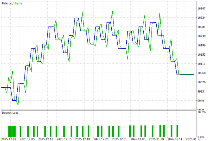
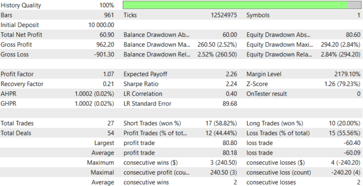
Models Back Test Results

 Looking at the backtest results below, we can see that integrating the Graph Neural Network–based liquidity detection into the trading system can identify tradable market structure zones, producing a positive net profit and profit factor above 1, which aligns with our goal of algorithmically detecting liquidity-driven opportunities. The back-testing was conducted on the XAUUSD pair, on the H1 timeframe across a 2-month testing window (01 December 2025 to 30 January 2026), with the default settings:

Conclusion

In summary, we addressed the challenge of identifying liquidity zones—areas where price is likely to react due to clustered orders—by combining graph-based machine learning with an automated trading system in MQL5. Instead of relying solely on traditional indicators or manual chart analysis, we transformed market structure into a graph representation, where swing highs and lows became nodes and their relationships formed edges. Using this structure, we trained a Graph Neural Network (GNN) to recognize patterns associated with liquidity accumulation. The trained model was then exported to ONNX format and integrated into an Expert Advisor, enabling the system to process live market data, construct graphs dynamically, run model inference, and detect potential liquidity zones directly within the trading platform.

In conclusion, this approach allows traders to enhance their systems with advanced pattern recognition capabilities that go beyond conventional technical analysis. By integrating machine learning with market structure analysis, traders can automate the detection of liquidity areas and use them to guide more informed trading decisions. When implemented within an automated strategy, this framework can help traders react faster to structural opportunities, reduce subjective bias in liquidity identification, and potentially improve the consistency of their trading systems by combining AI-driven insights with algorithmic execution.

File Name	Description
GNN for LqZs.ipynb	File containing the notebook to train and save the model.
ONNXRuntime.mqh	File containing the ONNXRuntime, which is our include file.
Graph NN.mq5	File containing the MQL5 EA, which loads the model and executes trades.
XAUUSD_H1.csv	File containing XAUUSD historical price data.