Optimal Trade Exit in MQL5: Longstaff-Schwartz Least-Squares Monte Carlo for Continuation-Value Estimation

Introduction

Every discretionary trader asks the same question about an open position: is this the best exit I'm going to get, or should I give it more room? Most automated systems answer with a fixed stop-loss/take-profit pair decided at entry, sometimes with a trailing rule bolted on - a reasonable default, but one that throws away information, since the market keeps talking after entry and a fixed level can't listen to any of it.

This article builds an exit engine that does listen. It borrows a tool from a different corner of quantitative finance: the Longstaff-Schwartz Least-Squares Monte Carlo (LSM) method, developed to price American options - contracts that, unlike European options, can be exercised any time before expiry. An open trading position shares that shape in one narrow sense: at every point you choose between exercising (closing the trade, banking what's on the table) and continuing (holding, keeping the optionality of a better price later). It isn't an option in any stricter sense - no counterparty, no risk-neutral price, and a losing position has a negative payoff a vanilla option never has. This article adapts that machinery - historical drift for risk-neutral valuation, position PnL net of costs for option payoff, an artificial forced-liquidation horizon for a fixed expiry - into a live trade-management module for MetaTrader 5.

Scope note: this project is a native MQL5 implementation - no ALGLIB, no external DLLs, no third-party libraries. The regression at the heart of LSM is solved with a hand-written, ridge-regularized Gauss-Jordan solver, described in full below. The default instrument and timeframe used throughout is XAUUSD M5, though nothing ties the engine to gold - it works from calibrated log-returns of whatever symbol and timeframe it is attached to.

What this engine actually decides: the LSM comparison below is primarily a profit-taking timer, not a hard stop-loss replacement. Its backward induction restricts the regression fit to in-the-money simulated paths, so it can bank a profit earlier than a full-horizon hold would - but the final comparison, between the real position's current payoff and the Monte Carlo continuation estimate, carries no equivalent restriction, so it can also signal an exit on a losing position when the simulated paths judge the expected outcome to be worse still (Fig. 3 shows exactly this). The two hard stop/backstop rules in the Expert Advisor section (a maximum holding period and a fixed stop-loss distance) remain in place as a bound that doesn't depend on the regression at all, acting independently of the LSM engine.

The system splits into four files with distinct responsibilities: a linear-algebra header, an engine header, an Expert Advisor, and an indicator. The indicator plots the exercise-versus-continuation decision so the logic is visible on the chart rather than buried in OnTick().

Position Exits as American Options

An American option gives its holder the right to exercise any time up to expiry, and the central pricing question is: at each point, is the payoff from exercising now bigger than the expected value of holding on? Longstaff and Schwartz answered this with a regression trick: simulate many forward paths, work backward from expiry, and at each step, for the "in-the-money" paths, regress the realized future cash flow on a handful of state variables - using the fit as the continuation value, compared against the immediate exercise payoff. Whichever is bigger determines the optimal action for that path at that step.

A live trading position maps onto this with one substitution worth noting: the valuation measure. Classic LSM discounts under a risk-neutral measure calibrated to option prices; here, simulation is calibrated from the instrument's own historical drift and volatility, producing a real-world expectation under the current regime - there's no market of counterparties to arbitrage against. The rest of the mapping holds: "underlying" is the instrument price, "strike" is the entry price, and "payoff from exercising" is the unrealized profit or loss if closed now, net of costs. The one piece that doesn't map directly is expiry - a trade has none, so the engine imposes an artificial one: a forced-liquidation horizon, InpLSMHorizonBars, past which everything is "must exit," giving the backward induction a well-defined terminal condition.

LSM Exit Decision Architecture

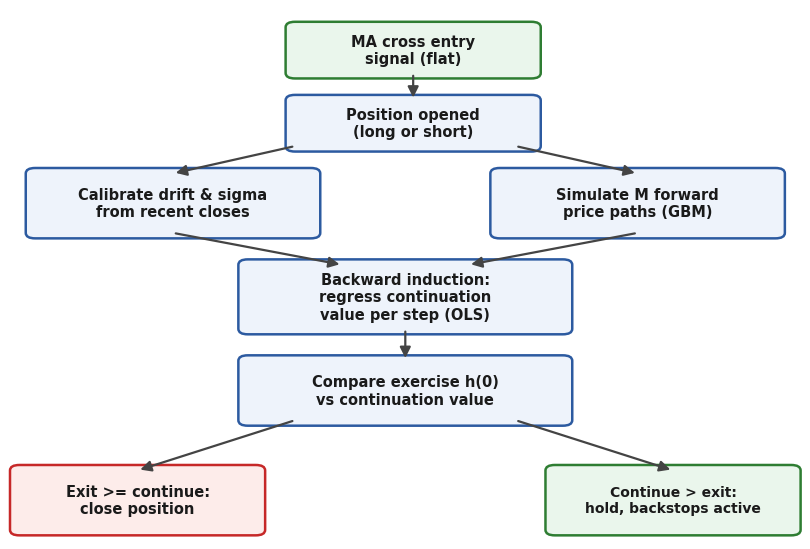
Fig. 1. The decision loop: entry, calibration, path simulation, backward induction, and the exercise-vs-continuation comparison that drives the exit.

While a position is open, the engine repeats the same four-stage loop on every check, with one exception in stage 1 noted below:

1. Calibrate drift and volatility from recent closes - done periodically, not on every tick.
2. Simulate a bundle of forward price paths from the current price.
3. Run backward induction over those paths to estimate the continuation value.
4. Compare the continuation value against the payoff of closing now, and act.

One design decision worth noting: the regression at each step only decides whether paths other than the real one would have stopped there, building up an estimate of what continuing is worth. The live position's current state is compared against that estimate once, at the very end, at step zero - the same way the original LSM algorithm prices an option.

Backward Induction: The Longstaff-Schwartz Regression

Write the exercise payoff at simulated step t on path i as h(t, i), and the discounted cash flow that path carries forward as CF(i). The backward induction EvaluateExit() implements walks from the second-to-last step down to step one

// for t = H-1 down to 1:
//   discount every path's CF one bar
//   ITM = { i : h(t,i) > 0 }
//   fit beta by regressing CF(i) on basis(t,i) for i in ITM
//   continuation_estimate(i) = basis(t,i) . beta
//   if h(t,i) >= continuation_estimate(i): CF(i) = h(t,i)   // exercise on this path
//   otherwise CF(i) is left as the discounted future cash flow

Two details make this more than a bookkeeping exercise. First, restricting the regression to in-the-money paths - the paths where the payoff is currently positive - is not an optimization, it is what makes the fit meaningful. A path that is deep out-of-the-money is never going to be a real exercise candidate at that step, and including it drags the regression toward describing states that are irrelevant to the actual decision boundary. This is exactly how Longstaff and Schwartz specify it in the original paper, and dropping it is a common way people accidentally rediscover a worse algorithm while believing they have implemented the same one.

Be precise about this: ExercisePayoff() can return a negative number, but inside the simulated backward induction the loop skips every path where pnl <= 0.0 before the regression comparison (`if(v <= 0.0) continue;` below), so a negative simulated payoff never enters the fit - exactly how Longstaff-Schwartz specify it, and harmless for a standard American option since a holder never exercises at a loss anyway. That restriction belongs to the simulated paths only, though: the final decision in EvaluateExit() compares the real position's current payoff against the resulting continuation estimate with no equivalent floor, so a negative current payoff can still clear that comparison if the continuation estimate is even more negative. This engine is primarily a profit-taking estimator asking "has this winner stopped being worth holding?" - but it isn't walled off from ever closing a loser, and Fig. 3 shows it doing exactly that. The two hard backstops in the Expert Advisor section remain the position's unconditional bound regardless of what the regression decides.

Second, the comparison at every interior step is local: it only asks whether each simulated path would have stopped there, never "should I exercise now" for the real position. That decision happens once, after the loop finishes, when the discounted average of all the CF(i) values - the Monte Carlo estimate of the continuation value - is compared against the real position's current payoff: what out_continue_value holds when EvaluateExit() returns.

A ridge penalty is added to the normal equations before every solve, since the number of in-the-money paths at a given step can be small relative to the six-term basis, and a small, poorly conditioned sample makes an un-regularized fit swing wildly. The ridge term shrinks the fit toward zero and keeps coefficients numerically sane without materially biasing a large, well-behaved sample.

Calibrating and Simulating the Forward Price Paths

The simulation needs two numbers before it can generate a single path: a per-bar drift and a per-bar volatility. Both are estimated from recent log-returns of the instrument and timeframe the EA runs on, rather than hardcoded, so the engine adapts as the regime changes. CalibrateFromHistory() does the estimation

   //+------------------------------------------------------------------+
   //| CalibrateFromHistory                                             |
   //| Estimates per-bar drift/volatility from recent closes;           |
   //|   returns false if too little history exists yet.                |
   //+------------------------------------------------------------------+
   bool CalibrateFromHistory(const string          symbol,
                              const ENUM_TIMEFRAMES tf,
                              const int             lookback_bars)
     {
      if(lookback_bars < 10)
         return(false);
      double closes[];
      ArraySetAsSeries(closes, true);
   //--- start at index 1 (not 0) so the still-forming current bar is
   //--- never folded into the calibration window - the same principle
   //--- ExportPriceHistory.mq5 applies to its own export, below
      int copied = CopyClose(symbol, tf, 1, lookback_bars, closes);
      if(copied < 10)
         return(false);
   //--- CopyClose fills a plain array chronologically (oldest to newest)
   //--- at the memory level - index 0 only means "most recent bar" once
   //--- ArraySetAsSeries(closes, true) is called BEFORE the copy, as
   //--- above. Skipping that call is the actual trap: the array still
   //--- compiles and returns data, just indexed the opposite way, which
   //--- silently flips the sign of every log-return computed from it -
   //--- log(closes[i] / closes[i+1]) is only the correct forward return
   //--- (older bar i+1 to newer bar i) because the array is explicitly
   //--- series-indexed here, not because of anything CopyClose does on
   //--- its own.
      int    n = copied - 1;
      double sum = 0.0;
      double returns[];
      ArrayResize(returns, n);
      for(int i = 0; i < n; i++)
        {
         returns[i] = MathLog(closes[i] / closes[i + 1]);
         sum       += returns[i];
        }
      double mean = sum / n;
      double sq_sum = 0.0;
      for(int i = 0; i < n; i++)
         sq_sum += (returns[i] - mean) * (returns[i] - mean);
   //--- sample variance (n-1 denominator) since this is an estimate
   //--- from a finite recent window, not the true population moment
      double variance = (n > 1) ? sq_sum / (n - 1) : 0.0;
      m_drift_per_bar = mean;
      m_sigma_per_bar = MathSqrt(MathMax(variance, 0.0));
      return(true);
     }

Starting the copy at index 1 rather than 0 matters for a second, separate reason beyond series-indexing: it keeps the still-forming current bar out of the calibration window - a partial, still-changing bar would otherwise feed a slightly different drift and volatility into the estimate on every recalibration, purely as an artifact of how far through that bar price happened to be at that instant. ExportPriceHistory.mq5 starts its own copy at index 1 for the same reason, further down.

Two modeling simplifications are worth noting. The simulated paths assume constant drift and volatility over the whole horizon and a log-normal return distribution - real intraday price action, especially on gold, clusters volatility and fattens its tails around news and session opens in ways a plain geometric Brownian motion never does, so these paths simplify the real process rather than forecast it. And a drift estimated from a short lookback window is itself a noisy number that can end up mattering more to the exit decision than it should, since little else in the basis counteracts it.

With drift and volatility in hand, EvaluateExit() generates the price paths themselves using standard geometric Brownian motion in log-returns:

double drift_term = m_drift_per_bar - 0.5 * m_sigma_per_bar * m_sigma_per_bar;
for(int p = 0; p < M; p++)
  {
   prices[p * (H + 1)] = current_price;
   for(int t = 1; t <= H; t++)
     {
      double z = NextStandardNormal();
      double prev = prices[p * (H + 1) + t - 1];
      //--- geometric Brownian motion step; using log-returns
      //--- guarantees simulated prices stay strictly positive,
      //--- which a naive additive random walk does not
      prices[p * (H + 1) + t] = prev * MathExp(drift_term + m_sigma_per_bar * z);
     }
  }

The standard normal draws feeding that loop come from a Box-Muller transform, generated in pairs and cached, since a single exit decision can call for tens of thousands of draws - InpLSMPaths times InpLSMHorizonBars. Box-Muller needs a uniform(0,1) source underneath it, and MQL5's native generator does not hand you one directly - there is no MathRandom() in real MQL5, an easy mistake to reach for out of habit, only MathRand(), which returns a pseudo-random integer in [0, 32767]:

   //+------------------------------------------------------------------+
   //| NextUniform01                                                    |
   //| Converts MathRand()'s integer [0, 32767] into a proper           |
   //|   half-open double [0, 1), dividing by 32768.0.                  |
   //+------------------------------------------------------------------+
   double NextUniform01(void)
     {
      return((double)MathRand() / 32768.0);
     }

With that in place, NextStandardNormal() itself is unchanged in structure - it still draws two uniforms and returns two normals, caching the second - only the source of those uniforms is now a real, compiling MQL5 call.

   //+------------------------------------------------------------------+
   //| NextStandardNormal                                               |
   //| Box-Muller: two uniform draws to two normal draws,               |
   //|   generated and cached in pairs to halve the call count.         |
   //+------------------------------------------------------------------+
   double NextStandardNormal(void)
     {
      if(m_has_spare_normal)
        {
         m_has_spare_normal = false;
         return(m_spare_normal);
        }

   //--- clamp away from exactly 0.0 to avoid MathLog(0) = -inf
      double u1 = MathMax(NextUniform01(), 1.0e-12);
      double u2 = NextUniform01();
      double r  = MathSqrt(-2.0 * MathLog(u1));
      double z0 = r * MathCos(2.0 * M_PI * u2);
      double z1 = r * MathSin(2.0 * M_PI * u2);

      m_spare_normal     = z1;
      m_has_spare_normal = true;
      return(z0);
     }

Forward Price Paths and Optimal Stopping Points

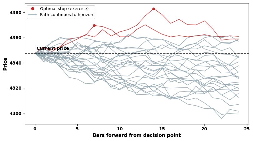
Fig. 2. A bundle of Monte Carlo forward paths generated by a direct port of the engine above, calibrated from a real 500-bar XAUUSD M5 export rather than an assumed volatility. Paths marked in red are the ones where the backward induction found an earlier bar preferable to holding to the horizon.

Fig. 2 shows a bundle after the backward induction has run over it, using drift and volatility computed directly from that real export - a per-bar drift of -0.0000311 and a per-bar sigma of 0.00092, reflecting the actual gold price decline over that window. Most paths simply drift to whatever the horizon forces, but a subset cross into territory where the regression judges immediate exercise better, marked with their stopping point.

Both figures above use real market data rather than an assumed volatility, which meant getting real closes out of the terminal first. That's a one-off job, not something the EA or indicator need to do themselves, so it lives in a small standalone Script rather than the trio above.

ExportPriceHistory.mq5

//+------------------------------------------------------------------+
//| OnStart                                                          |
//+------------------------------------------------------------------+
// Exports InpBarCount closed bars of InpSymbol/InpTF as (time, close)
// rows to a CSV in the shared Common\Files folder. This is a one-off
// analysis tool, not part of the EA/indicator/include trio - it exists
// only to feed real calibration data into an offline Python
// reproduction of CLSMExitEngine, and is not itself attached to a
// chart or run repeatedly.
void OnStart(void)
  {
   string symbol = (InpSymbol == "") ? _Symbol : InpSymbol;
//--- shift the copy start index by 1 so the export begins at the last
//--- fully CLOSED bar, never the still-forming current bar - starting
//--- at index 0 would make the export's last row silently change
//--- every time the script is re-run intraday
   datetime times[];
   double   closes[];
   int copied_t = CopyTime(symbol, InpTF, 1, InpBarCount, times);
   int copied_c = CopyClose(symbol, InpTF, 1, InpBarCount, closes);
   int n = MathMin(copied_t, copied_c);
   if(n < InpBarCount)
      Print("OnStart: only ", n, " of ", InpBarCount,
            " requested bars are available in history - exporting what is there");
   if(n <= 0)
     {
      Print("OnStart: no history available for ", symbol, " on the requested timeframe");
      return;
     }
//--- neither times[] nor closes[] is switched into series mode here,
//--- so CopyTime/CopyClose fill them the plain way: index 0 is the
//--- OLDEST bar in the requested range, and the last index is the
//--- most recent closed bar. The file is written out in that same
//--- oldest-first order, which is what a CSV meant to be read top to
//--- bottom in chronological order should look like - note that this
//--- is the opposite convention from CalibrateFromHistory() in
//--- LSMEngine.mqh, which explicitly series-indexes its own copy so
//--- index 0 means "most recent" there instead
   string filename = "LSMTradeExit_PriceExport_" + symbol + ".csv";
   int handle = FileOpen(filename, FILE_WRITE | FILE_CSV | FILE_COMMON | FILE_ANSI, ',');
   if(handle == INVALID_HANDLE)
     {
      Print("OnStart: failed to open ", filename, ", error ", GetLastError());
      return;
     }
   FileWrite(handle, "time", "close");
   for(int i = 0; i < n; i++)
      FileWrite(handle, TimeToString(times[i], TIME_DATE | TIME_MINUTES | TIME_SECONDS),
                DoubleToString(closes[i], _Digits));
   FileClose(handle);
   Print("OnStart: exported ", n, " bars of ", symbol, " to Common\\Files\\", filename);
  }

Run once on an XAUUSD M5 chart with enough history loaded, this is exactly what produced the 500-bar export that Fig. 2 and Fig. 3 are calibrated from and walked through. It writes to the shared Common\\Files folder, the same convention the EA's own diagnostics log uses, so the export survives terminal reinstalls and any offline script can find it without guessing which terminal instance produced it.

Basis Functions and the Native OLS Solver

The regression basis is what the continuation-value estimate depends on. Too few terms and the fit can't capture the decision boundary's shape; too many and it overfits the modest in-the-money sample at early steps. Six terms strikes that balance: an intercept, the payoff, its square (curvature near the boundary, as in the original Longstaff-Schwartz basis), the fraction of horizon elapsed, the best payoff seen so far, and a payoff/time interaction

   //+------------------------------------------------------------------+
   //| BuildBasisRow                                                    |
   //| Basis functions at one path/time step, matching SolveOLS's       |
   //|   fixed X[][6] layout: 1.0, pnl_now, pnl_now^2 (curvature, as in |
   //|   the original LS basis), time_frac, peak_pnl (best payoff so    |
   //|   far), and pnl_now*time_frac (payoff/time interaction).         |
   //+------------------------------------------------------------------+
void BuildBasisRow(const double pnl_now,
                       const double peak_pnl,
                       const double time_frac,
                       double      &row[]) const
     {
      ArrayResize(row, 6);
      row[0] = 1.0;
      row[1] = pnl_now;
      row[2] = pnl_now * pnl_now;
      row[3] = time_frac;
      row[4] = peak_pnl;
      row[5] = pnl_now * time_frac;
     }

The fourth term - the running peak of the payoff along a path - is a cheap stand-in for a trailing or drawdown-from-peak effect, without carrying the full path history as a state variable. A path that ran up to +40 points and has since faded to +10 is a meaningfully different state from one that has only ever been at +10, even though the instantaneous payoff is identical, and this term lets the regression tell the two apart.

Worth being clear about: this peak-tracking only exists inside each simulated future path. The real position's own trading history - whatever maximum unrealized profit it already reached - is not an input to EvaluateExit() at all; the comparison at step zero never sees the real trade's own trailing high, only the raw current exercise payoff against the Monte Carlo average.

Fitting those six coefficients at every backward step is a small least squares problem, solved with a hand-rolled, ridge-regularized Gauss-Jordan elimination rather than any external library. The design matrix is built from the basis rows of the in-the-money paths, and the target vector is each path's discounted realized cash flow

//+------------------------------------------------------------------+
//| SolveOLS                                                         |
//| Fits beta in y ~ X*beta via ridge-regularized Gauss-Jordan:      |
//|   (X'X + lambda*I)*beta = X'y. Returns false (caller falls back  |
//|   to "always continue") if the system couldn't be pivoted.       |
//+------------------------------------------------------------------+
bool SolveOLS(const double &X[][6],
              const double &y[],
              const int     rows,
              const int     cols,
              const double  lambda,
              double       &beta[])
  {
//--- guard: require at least as many in-the-money paths as basis
//--- terms. Ridge regularization can, in principle, still produce a
//--- solution with fewer rows than columns, so this is a deliberate
//--- reliability choice rather than a mathematical necessity - a fit
//--- built from fewer observations than free parameters is not
//--- trusted to drive a real exit decision here, whatever it solves to
   if(rows < cols)
      return(false);

//--- build the symmetric cols x cols Gram matrix XtX and the
//--- cols-length vector Xty by direct summation; this is the
//--- classic normal-equation formulation, cheap here because cols
//--- is fixed and small (the basis has at most 6 terms)
   double xtx[6][6];
   double xty[6];
   for(int a = 0; a < cols; a++)
     {
      xty[a] = 0.0;
      for(int b = 0; b < cols; b++)
         xtx[a][b] = 0.0;
     }

   for(int r = 0; r < rows; r++)
     {
      for(int a = 0; a < cols; a++)
        {
         //--- accumulate X'y for this row's contribution
         xty[a] += X[r][a] * y[r];
         for(int b = 0; b < cols; b++)
            xtx[a][b] += X[r][a] * X[r][b];
        }
     }

//--- add the ridge penalty to the diagonal only; this shrinks the
//--- coefficients toward zero and, critically, guarantees a
//--- strictly positive diagonal even when a basis column is nearly
//--- collinear with another (e.g. pnl and pnl^2 on a narrow path
//--- sample), which is what actually causes Gauss-Jordan to fail
   for(int a = 0; a < cols; a++)
      xtx[a][a] += lambda;

The solver builds the Gram matrix X'X and the vector X'y from direct summation, adds the ridge penalty to the diagonal only, then eliminates with partial pivoting - swapping in whichever remaining row has the largest absolute entry in the pivot column, so the elimination never divides by something close to zero

   double eps = 1.0e-12;
   for(int col = 0; col < cols; col++)
     {
      int    pivot_row = col;
      double pivot_val = MathAbs(aug[col][col]);
      for(int r = col + 1; r < cols; r++)
        {
         if(MathAbs(aug[r][col]) > pivot_val)
           {
            pivot_val = MathAbs(aug[r][col]);
            pivot_row = r;
           }
        }
      if(pivot_val < eps)
         return(false);            //--- system too degenerate to trust

      if(pivot_row != col)
        {
         for(int c = 0; c <= cols; c++)
           {
            double tmp        = aug[col][c];
            aug[col][c]       = aug[pivot_row][c];
            aug[pivot_row][c] = tmp;
           }
        }

      //--- normalize the pivot row so aug[col][col] becomes 1.0
      double piv = aug[col][col];
      for(int c = 0; c <= cols; c++)
         aug[col][c] /= piv;

      //--- eliminate this column from every other row (full
      //--- Gauss-Jordan, not just below the pivot) so the final
      //--- augmented column is the solution directly, with no
      //--- separate back-substitution pass required
      for(int r = 0; r < cols; r++)
        {
         if(r == col)
            continue;
         double factor = aug[r][col];
         for(int c = 0; c <= cols; c++)
            aug[r][c] -= factor * aug[col][c];
        }
     }

Two failure modes are handled explicitly rather than left to produce garbage silently. If there are fewer in-the-money paths than basis terms, SolveOLS() refuses outright - a deliberate reliability choice, since a fit built from fewer observations than free parameters is not trusted to drive a real exit decision. If every candidate pivot in a column is smaller than 1.0e-12, the function also returns false, signalling a degenerate fit. In both cases EvaluateExit() simply skips updating the cash flows for that step, equivalent to assuming "continue" was optimal there - cautious in that it never lets an unreliable regression invent an exercise decision, but not the safer outcome for a currently losing position, which risks letting the loss run rather than cutting it. "Do not trust a degenerate fit" is a more accurate description of this fallback than "the conservative choice."

Two further limitations: the six basis terms aren't scaled to comparable magnitudes before the ridge penalty applies, so a fixed lambda doesn't shrink every coefficient equally. And forming the normal equations X'X is numerically harder than solving via QR or SVD, since squaring the design matrix roughly squares its condition number - ridge keeps Gauss-Jordan from failing outright, but doesn't make this as stable as a factorization-based solver.

Assembling the CLSMExitEngine Class

With the simulation, basis, and solver pieces in place, the rest of the class is mostly plumbing: a payoff function, a constructor with safe defaults, and a configuration method turning a nominal annual discount rate into the per-bar discount factor the backward induction uses

   //+------------------------------------------------------------------+
   //| ExercisePayoff                                                   |
   //| Payoff of closing now at 'price', net of an estimated            |
   //|   round-trip cost. Direction-aware: a long profits as price      |
   //|   rises above entry, a short as it falls below entry.            |
   //+------------------------------------------------------------------+
   double ExercisePayoff(const double price,
                          const double entry_price,
                          const long   pos_type,
                          const double cost_points) const
     {
      double raw = (pos_type == POSITION_TYPE_BUY)
                   ? (price - entry_price)
                   : (entry_price - price);
      return(raw - cost_points);
     }

Keeping this single, small function as the only place that computes a payoff means the simulation, the regression targets, and the live exercise decision all use an identical definition of profit - no rounding or sign inconsistency can creep in between them.

One simplification worth noting: current_price is already the bid for a long or ask for a short, so spread is partly embedded in the payoff before cost_points is even subtracted. If cost_points also includes the full spread, part is double-counted - InpCostPoints here approximates commission and slippage on top of it, but a production version would break spread, commission, swap, and slippage into distinct terms.

Configure() converts a nominal annual discount rate into a per-bar factor using the chart's own timeframe

   //+------------------------------------------------------------------+
   //| Configure                                                        |
   //| paths, horizon_bars, ridge_lambda : Monte Carlo path count,      |
   //|   forced-liquidation horizon, and ridge penalty (passed          |
   //|   straight through to SolveOLS). annual_rate / bar_seconds :     |
   //|   derive the per-bar discount factor, kept near-neutral since    |
   //|   intraday horizons make time value negligible.                  |
   //+------------------------------------------------------------------+
   void Configure(const int    paths,
                  const int    horizon_bars,
                  const double ridge_lambda,
                  const double annual_rate,
                  const int    bar_seconds)
     {
      m_paths        = MathMax(paths, 50);
      m_horizon_bars = MathMax(horizon_bars, 2);
      m_ridge_lambda = MathMax(ridge_lambda, 0.0);

   //--- convert an annual rate to a per-bar discount factor;
   //--- seconds_per_year uses 252 trading days to stay consistent
   //--- with how the rest of the series annualizes intraday figures
      double seconds_per_year = 252.0 * 24.0 * 60.0 * 60.0;
      double bar_fraction     = (double)bar_seconds / seconds_per_year;
      m_discount_per_bar      = MathExp(-annual_rate * bar_fraction);
     }

The default InpAnnualRate is zero, which makes m_discount_per_bar exactly 1.0 - discounting is effectively switched off. That is deliberate: over a horizon of a few dozen five-minute bars, the time value of money is not a meaningful driver of the exit decision, and forcing a nonzero rate onto a short intraday horizon would add noise without insight. The mechanism stays in, faithful to the original discounted-cashflow formulation, in case anyone adapts this to a much longer holding-period exit.

The rest of EvaluateExit() is the loop that pre-computes payoff and running-peak arrays once per path, initializes the terminal cash flow, and then, at every backward step, gathers the in-the-money paths into a design matrix and calls the solver. Its signature is worth a closer look first, since the bars_remaining parameter closes a real gap worth naming directly:

   //+------------------------------------------------------------------+
   //| EvaluateExit                                                     |
   //| Runs one LSM pass; true if immediate exercise beats              |
   //|   continuation. current_price/entry_price/pos_type/cost_points : |
   //|   live quote, open price, direction, cost. bars_remaining : H =  |
   //|   MathMin(m_horizon_bars, bars_remaining). out_exercise_value /  |
   //|   out_continue_value : h(0) and continuation; true when exercise |
   //|   >= continue.                                                   |
   //+------------------------------------------------------------------+
   bool EvaluateExit(const double current_price,
                      const double entry_price,
                      const long   pos_type,
                      const double cost_points,
                      const int    bars_remaining,
                      double      &out_exercise_value,
                      double      &out_continue_value)
     {
   //--- shrink the simulated horizon toward the real deadline as the
   //--- position ages - capped at bars_remaining in every case, with
   //--- no floor that could push it back above the real deadline
      int H = MathMin(m_horizon_bars, bars_remaining);
      int M = m_paths;

The key parameter is bars_remaining. If a full horizon is simulated on every call, the continuation value retains "fresh optionality" and rarely loses to hard backstops. Clamping the simulated horizon to bars_remaining makes the continuation value decay as the real deadline approaches, and it does so in a strict sense: H is never above bars_remaining, full stop, with no floor that could push it back above the real deadline. A very small bars_remaining near the deadline still simulates safely without that floor - it just produces a shorter, noisier backward induction, and the existing per-step guards (too few in-the-money paths, or a degenerate regression) already fall back to "continue" gracefully rather than fitting something unreliable, so there is nothing extra needed to handle the small-horizon case safely.

With the horizon clamped this way, the rest of the backward-induction loop is straightforward: gather the in-the-money paths at each step into a design matrix, and hand it to the solve

         int itm_count = 0;
         for(int p = 0; p < M; p++)
            if(pnl[p * (H + 1) + t] > 0.0)
               itm_count++;

         if(itm_count < 8)
            continue;              //--- too few ITM paths - skip this
                                    //--- step's update and implicitly
                                    //--- treat it as "always continue"
                                    //--- rather than fit an unreliable
                                    //--- regression on a handful of points

         double X[][6];
         double y[];
         ArrayResize(X, itm_count);
         ArrayResize(y, itm_count);

         int    idx[];
         ArrayResize(idx, itm_count);
         int    row = 0;
         double time_frac = (double)t / (double)H;
         for(int p = 0; p < M; p++)
           {
            double v = pnl[p * (H + 1) + t];
            if(v <= 0.0)
               continue;
            double basis[];
            BuildBasisRow(v, peak[p * (H + 1) + t], time_frac, basis);
            for(int c = 0; c < 6; c++)
               X[row][c] = basis[c];
            y[row] = cf[p];
            idx[row] = p;
            row++;
           }

         double beta[];
         bool ok = SolveOLS(X, y, itm_count, 6, m_ridge_lambda, beta);
         if(!ok)
            continue;              //--- degenerate fit - same fallback
                                    //--- as the too-few-paths case above

Once a regression succeeds for a step, the fitted coefficients are evaluated against every in-the-money path's own basis row, and cf[] is overwritten in place wherever exercising beats the estimate - this is the step that actually discovers each path's optimal stopping time, working backward one step at a time.

         for(int r = 0; r < itm_count; r++)
           {
            int p = idx[r];
            double basis[];
            BuildBasisRow(pnl[p * (H + 1) + t], peak[p * (H + 1) + t], time_frac, basis);
            double continuation_est = 0.0;
            for(int c = 0; c < 6; c++)
               continuation_est += basis[c] * beta[c];

            if(pnl[p * (H + 1) + t] >= continuation_est)
               cf[p] = pnl[p * (H + 1) + t];
           }
        }

After the loop reaches step one, the cash flows are discounted one final bar to bring them back to "now" and averaged - that average is the Monte Carlo estimate of out_continue_value - and compared against the real position's current exercise payoff to produce the boolean the caller acts on

      double sum_cf = 0.0;
      for(int p = 0; p < M; p++)
         sum_cf += cf[p] * m_discount_per_bar;
      out_continue_value = sum_cf / M;

      out_exercise_value = ExercisePayoff(current_price, entry_price, pos_type, cost_points);

      return(out_exercise_value >= out_continue_value);
     }

The Expert Advisor: Entry Signal and Exit Integration

The entry side of the EA is intentionally simple: a fast/slow moving-average cross, recomputed from scratch on every call via CopyBuffer() rather than cached. This is a deliberate choice for the article, not a claim that MA crosses are a good standalone strategy - the entry logic is held constant so the LSM exit engine is the only variable under test

//+------------------------------------------------------------------+
//| GetEntrySignal                                                   |
//| Reads the two MA buffers on the last two closed bars; returns    |
//|   +1/-1 for a fresh cross, 0 otherwise. Recomputed from scratch  |
//|   via CopyBuffer every call, so it can't drift from the chart.   |
//+------------------------------------------------------------------+
int GetEntrySignal(void)
  {
   double fast[], slow[];
   ArraySetAsSeries(fast, true);
   ArraySetAsSeries(slow, true);

   if(CopyBuffer(g_fast_ma_handle, 0, 0, 3, fast) < 3)
      return(0);
   if(CopyBuffer(g_slow_ma_handle, 0, 0, 3, slow) < 3)
      return(0);

//--- compare the two most recently CLOSED bars (index 1 vs 2),
//--- never the still-forming bar at index 0, to avoid acting on a
//--- cross that can still repaint before the bar closes
   bool was_below = fast[2] <= slow[2];
   bool now_above = fast[1] >  slow[1];
   bool was_above = fast[2] >= slow[2];
   bool now_below = fast[1] <  slow[1];

   if(was_below && now_above)
      return(1);
   if(was_above && now_below)
      return(-1);
   return(0);
  }

The exit side is where the LSM engine plugs in, but it is never the only thing standing between the account and an open-ended loss. Two hard backstops - a maximum holding period and a fixed stop-loss distance - are checked first, independent of whether the LSM engine is even working correctly that tick

//+------------------------------------------------------------------+
//| CheckLSMExit                                                     |
//| Runs the LSM engine; closes the position if immediate            |
//|   exercise beats continuation. Horizon shrinks toward            |
//|   InpMaxHoldingBars as the position ages; a max holding period   |
//|   and fixed stop-loss act as hard backstops.                     |
//+------------------------------------------------------------------+
void CheckLSMExit(void)
  {
   long     pos_type;
   double   entry_price;
   datetime open_time;
   if(!HasOpenPosition(pos_type, entry_price, open_time))
      return;

//--- backstop 1: hard time-based liquidation, independent of LSM
   int bars_held = iBarShift(_Symbol, _Period, open_time, false);
   if(bars_held >= InpMaxHoldingBars)
     {
      g_trade.PositionClose(_Symbol);
      LogDecision(entry_price, entry_price, 0.0, "BACKSTOP_TIME");
      return;
     }

//--- backstop 2: hard price-based stop, independent of LSM
   double bid = SymbolInfoDouble(_Symbol, SYMBOL_BID);
   double ask = SymbolInfoDouble(_Symbol, SYMBOL_ASK);
   double point = SymbolInfoDouble(_Symbol, SYMBOL_POINT);
   double current_price = (pos_type == POSITION_TYPE_BUY) ? bid : ask;

   double adverse_move = (pos_type == POSITION_TYPE_BUY)
                          ? (entry_price - current_price)
                          : (current_price - entry_price);
   if(adverse_move >= InpBackstopSLPts * point)
     {
      g_trade.PositionClose(_Symbol);
      LogDecision(current_price, current_price, 0.0, "BACKSTOP_SL");
      return;
     }

//--- periodic recalibration begins below: counted in real closed bars,
//--- not in ticks or calls to this function

This ordering matters. If the regression solver were ever to fail repeatedly, the LSM engine would simply keep returning "continue" by its own conservative fallback, and without the two backstops above, a position could theoretically be held indefinitely. The time-based and price-based backstops close that gap without depending on the LSM machinery working at all.

Once those pass, the engine recalibrates periodically - not every tick, since drift and volatility barely change tick to tick. CheckLSMExit() runs once per tick, though, so the bar count has to be derived rather than assumed: a static s_last_calib_bar_time compares the current bar's open time against the last one seen, and g_bars_since_calib only advances on a new closed bar. Without that guard, InpRecalibEveryN would silently mean "every N ticks" rather than "every N bars" - shorter on a fast-ticking symbol. With the guard in place, EvaluateExit() is called and its verdict logged and acted on.

   //--- gate the counter on an actual new closed bar - without this,
   //--- g_bars_since_calib counts calls to CheckLSMExit(), which runs
   //--- every tick, not every bar, and InpRecalibEveryN would silently
   //--- mean "every N ticks" instead of "every N bars"
   static datetime s_last_calib_bar_time = 0;
   datetime current_bar_time = iTime(_Symbol, _Period, 0);
   if(current_bar_time != s_last_calib_bar_time)
     {
      s_last_calib_bar_time = current_bar_time;
      g_bars_since_calib++;
      if(g_bars_since_calib >= InpRecalibEveryN)
         {
          g_engine.CalibrateFromHistory(_Symbol, _Period, InpCalibLookback);
          g_bars_since_calib = 0;
         }
     }

   double cost_points = InpCostPoints * point;
   int bars_remaining = InpMaxHoldingBars - bars_held;    //--- guaranteed > 0
                                                          //--- here: backstop 1
                                                          //--- above already
                                                          //--- returned if
                                                          //--- bars_held reached
                                                          //--- InpMaxHoldingBars
   double exercise_value, continue_value;
   bool should_exit = g_engine.EvaluateExit(current_price, entry_price, pos_type,
                                            cost_points, bars_remaining,
                                            exercise_value, continue_value);

   LogDecision(exercise_value, continue_value, current_price,
               should_exit ? "LSM_EXIT" : "LSM_HOLD");

   if(should_exit)
      g_trade.PositionClose(_Symbol);
  }

bars_remaining is computed as InpMaxHoldingBars - bars_held, always positive by this point since backstop 1 already returned early otherwise. That single value makes the LSM comparison time-aware: early in a trade's life it is large and the continuation value reflects a genuinely long look-ahead; as the position ages, it shrinks toward the immediate exercise payoff - behaviour Fig. 3 in the next section shows.

Every decision - backstop trigger or LSM verdict - is written to a CSV log via LogDecision(), opened once in OnInit() with FILE_COMMON so it survives terminal reinstalls and lands where any offline Python script can read it. Encoding note: MQL5 FILE_CSV defaults to UTF-16 - Python must open it with encoding="utf-16", or the text garbles without a clear error.

The Continuation Monitor Indicator

A CSV log is precise but not immediate - reading it means opening a spreadsheet afterward. LSM_ContinuationMonitor.mq5 plots the same two numbers the EA compares, live, in a separate chart window, running its own EvaluateExit() call with the same Configure() parameters every bar close

//+------------------------------------------------------------------+
//| OnCalculate                                                      |
//| Only recomputes the most recently closed bar (index 1), not      |
//|   the whole history every tick - each LSM pass is a full sim     |
//|   plus backward induction. Middle-of-history bars stay           |
//|   EMPTY_VALUE - this is a monitor, not a backtesting overlay.    |
//+------------------------------------------------------------------+
int OnCalculate(const int        rates_total,
                 const int        prev_calculated,
                 const datetime  &time[],
                 const double    &open[],
                 const double    &high[],
                 const double    &low[],
                 const double    &close[],
                 const long      &tick_volume[],
                 const long      &volume[],
                 const int       &spread[])
  {
   if(rates_total < 2)
      return(0);

//--- recalibrate once per call rather than caching across calls;
//--- this indicator only recomputes on new closed bars anyway (see
//--- the static guard below), so the extra CalibrateFromHistory
//--- cost is paid at most once per bar
   g_engine.CalibrateFromHistory(_Symbol, _Period, InpCalibLookback);

   static datetime last_processed = 0;
   datetime this_bar_time = time[rates_total - 1];
   if(this_bar_time == last_processed)
      return(rates_total);
   last_processed = this_bar_time;

The static last_processed guard is what keeps this usable: re-running a full Monte Carlo pass on every incoming tick, rather than once per closed bar, would make the chart lag rather than help. Bars where no matching position exists, or where the calculation has not yet run, are left as EMPTY_VALUE. Because this indicator tracks the same decision the EA is making, it computes bars_remaining the same way CheckLSMExit() does - mirroring InpMaxHoldingBars as an input, and reading the position's own open time.

"Mirrors" is the right word, not "guarantees a match." Two things keep the indicator's plot from matching the EA exactly: it recalibrates every bar, while the EA only recalibrates every InpRecalibEveryN bars; and EvaluateExit() draws fresh random paths every call, so identical inputs still give two independent samples of the same estimator - a close approximation of what the EA sees, not a deterministic replay.

   long   pos_type      = PositionGetInteger(POSITION_TYPE);
   double entry_price   = PositionGetDouble(POSITION_PRICE_OPEN);
   datetime open_time   = (datetime)PositionGetInteger(POSITION_TIME);
   double point         = SymbolInfoDouble(_Symbol, SYMBOL_POINT);
   double bid           = SymbolInfoDouble(_Symbol, SYMBOL_BID);
   double ask           = SymbolInfoDouble(_Symbol, SYMBOL_ASK);
   double current_price = (pos_type == POSITION_TYPE_BUY) ? bid : ask;
   double cost_points   = InpCostPoints * point;

//--- mirror the EA's own bars_remaining computation exactly, so the
//--- plotted continuation value matches what the EA itself would
//--- have used for the same position at the same bar
   int bars_held      = iBarShift(_Symbol, _Period, open_time, false);
   int bars_remaining = MathMax(1, InpMaxHoldingBars - bars_held);

   double exercise_value, continue_value;
   g_engine.EvaluateExit(current_price, entry_price, pos_type, cost_points,
                          bars_remaining, exercise_value, continue_value);

Exercise Value vs. LSM Continuation Value

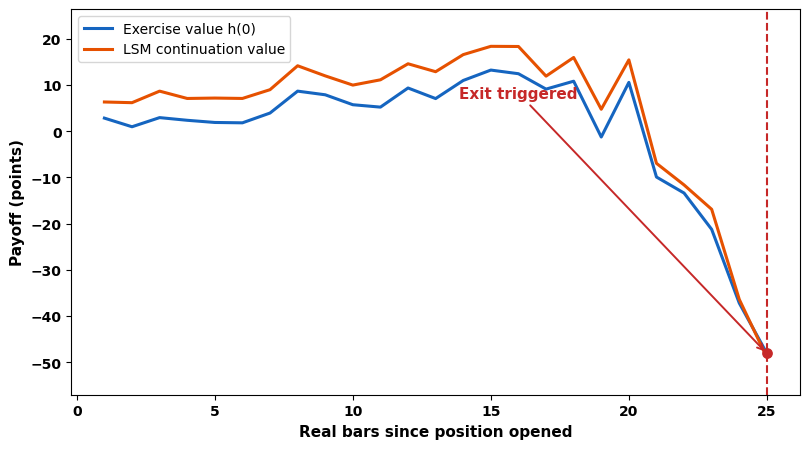
Fig. 3. A run of the ported algorithm over an actual historical XAUUSD M5 price path, walked bar by bar with a 96-bar maximum holding period and recalibrated from the real trailing window at every step. Where the exercise line crosses the continuation line is the bar at which this replay's own draws judge immediate exercise better than continuing - a close approximation of a live run, not a guaranteed match.

Fig. 3 is not a stylized illustration - it is the actual Longstaff-Schwartz engine, re-implemented line-for-line in Python from LSMEngine.mqh, called once per bar using the same EvaluateExit() logic CheckLSMExit() calls (recalibrating every step here, not only every InpRecalibEveryN bars, for a more responsive replay). The short position shown opens favorably, its continuation value climbing for the first fifteen bars to peak around +18 points - then the real market reverses hard, and both lines fall together, the exercise line crossing above the continuation line at bar 25 as the loss approaches -48 points. That crossover is driven by the real reversal, not the horizon floor: with fresh calibration every step, a sharp move against the position is exactly what this comparison catches.

The remaining function, OnInit(), binds the two plot buffers and calls Configure() with parameters that intentionally mirror the EA's own inputs, so a chart running both together is comparing like with like.

//+------------------------------------------------------------------+
//| OnInit                                                           |
//| Binds the two plot buffers and configures the LSM engine with the|
//| same parameters as the EA so the plotted values are directly     |
//| comparable to what actually drove any historical exit.           |
//+------------------------------------------------------------------+
int OnInit(void)
  {
   SetIndexBuffer(0, g_exercise_buf, INDICATOR_DATA);
   SetIndexBuffer(1, g_continue_buf, INDICATOR_DATA);
   ArraySetAsSeries(g_exercise_buf, true);
   ArraySetAsSeries(g_continue_buf, true);
   PlotIndexSetDouble(0, PLOT_EMPTY_VALUE, EMPTY_VALUE);
   PlotIndexSetDouble(1, PLOT_EMPTY_VALUE, EMPTY_VALUE);

   int bar_seconds = PeriodSeconds(_Period);
   g_engine.Configure(InpLSMPaths, InpLSMHorizonBars, InpRidgeLambda,
                       InpAnnualRate, bar_seconds);

   return(INIT_SUCCEEDED);
  }

Edge Cases and Pitfalls

Cold-start calibration. CalibrateFromHistory() is called once in OnInit() so the first check never runs against zeroed defaults. With fewer than ten bars of history, calibration returns false and the engine keeps its last estimate - on a brand-new symbol, a flat, zero-drift assumption. Safe (every path becomes a straight line, so continuation value collapses toward current payoff) but not useful, so the EA leans on its backstops until enough history accumulates.

Regime shift mid-trade. Drift and volatility only recalibrate every InpRecalibEveryN bars, not every tick, so a position opened just before a sharp volatility spike will simulate for several bars against stale calibration, understating how far price could move. Shortening InpRecalibEveryN reduces this lag at the cost of more frequent history reads.

Ridge lambda sensitivity. Too small reintroduces the instability it's meant to prevent on thin in-the-money samples; too large flattens every regression toward a constant, defeating the point of running LSM over a simpler rule. InpRidgeLambda defaults to 1e-6, a safety net rather than a tuning lever.

Monte Carlo noise. EvaluateExit() draws fresh random paths every call, so two consecutive calls on an unchanged position can return slightly different continuation-value estimates. At the default InpLSMPaths of 500 this noise is small, but the exact exit bar isn't perfectly deterministic - raising the path count reduces variance at a roughly linear CPU cost.

Strategy Tester sandboxing. The CSV log uses FILE_COMMON, resolving to the shared Common\Files folder rather than the terminal's own MQL5\Files - necessary since each Tester agent runs in an isolated Files sandbox separate from the live terminal, where a log written only locally wouldn't be visible to it.

Testing in the Strategy Tester

The exit engine is a mechanism, not a strategy, and testing it once on one symbol and timeframe would only tell part of the story. Four real Strategy Tester runs are reported below - all-tick modeling, 100% history quality, the same six-month window, MA-cross entry logic, and EA defaults untouched throughout - covering a metal and three major forex pairs across four timeframes: XAUUSD M5, EURUSD M15, GBPUSD H1, and USDJPY M30.

Note on methodology: InpLSMHorizonBars, InpMaxHoldingBars, and InpBackstopSLPts are all counted in bars and points, not real time or volatility-normalized distance. The same 24-bar horizon is 2 hours on M5 and a full day on H1; the same 600-point backstop is a very different move on XAUUSD than on a 5-decimal forex pair. None of the four runs re-tuned these per timeframe - reported exactly as shipped, itself part of the finding.

Metric	XAUUSD M5	EURUSD M15	GBPUSD H1	USDJPY M30
Total net profit	-$5,946.70	+$829.40	-$829.00	+$785.40
Profit factor	0.87	1.73	0.50	1.84
Expected payoff	-$8.47	+$8.92	-$22.41	+$17.07
Sharpe ratio	-2.28	3.11	-2.96	2.22
Recovery factor	-0.66	2.61	-0.92	2.09
Max equity drawdown	69.87%	2.92%	8.96%	3.51%
Win rate	13.39% (94/702)	56.99% (53/93)	27.03% (10/37)	47.83% (22/46)
Average win / loss	$416.29/-$74.14	$37.22/-$28.58	$84.34/-$61.94	$78.30/-$39.05
Total trades	702	93	37	46

XAUUSD M5 Balance and Equity Curve

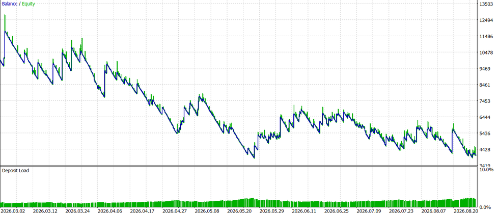
Fig. 4. The balance/equity curve for the XAUUSD M5 run specifically - the largest sample of the four (702 trades) and the one with the deepest drawdown, unedited apart from cropping the terminal chrome.

By profit factor and Sharpe ratio - the metrics least distorted by the different trade counts and currency-per-point values - GBPUSD H1 is the weakest of the four (0.50 profit factor, -2.96 Sharpe), worse on both counts than XAUUSD M5 despite losing less money outright, simply because far fewer trades were taken (37 versus 702). XAUUSD M5 loses the most money and carries the worst drawdown, 69.87%. EURUSD M15 and USDJPY M30 both come back solidly profitable - profit factors of 1.73 and 1.84, Sharpe ratios above 2, drawdowns under 4%. None of this is a clean ranking, though: given the unequal settings already flagged, these results read better side by side than ordered against one another.

Two symbols losing money and two making it, on the same code with the same untouched settings, is itself the headline result - though these runs don't isolate exit-mechanism quality from entry/risk settings, since there's no baseline with a fixed stop-loss/take-profit, trailing stop, or plain time exit in place of the LSM engine. Trade count scales inversely with timeframe (702 on M5 down to 37 on H1), leaving H1 on a much thinner sample from a stochastic engine whose output carries run-to-run noise. GBPUSD H1 illustrates the methodology note's warning directly: a 24-bar horizon is a full day on H1, and a 600-point backstop is tight for that timeframe - never tuned for it, and it shows.

"This works" or "this does not work" is the wrong question for these four runs - exit-engine quality and entry/parameter quality are entangled, and separating them cleanly would need a fixed-risk-per-trade sizing scheme and per-timeframe horizon tuning, neither of which this test isolates. That's a natural next step, not something to paper over. The CSV log, the continuation-monitor indicator, and this table show the mechanism runs and produces a coherent, inspectable decision at every bar; none of the three is evidence it improves trading outcomes over a simpler exit.

Conclusion

This article repurposed Longstaff-Schwartz's regression-based continuation-value estimate for live exit management: historical drift in place of risk-neutral dynamics, position PnL net of costs for option payoff, an artificial forced-liquidation horizon for a fixed expiry - with a native Gauss-Jordan solver and a small basis of state variables (payoff, its square, elapsed time, running peak, and their interaction). The regression that builds the continuation estimate is fit only on in-the-money simulated paths, but the final comparison against the real position's own payoff carries no such restriction - so alongside deciding when to take a profit, it can also close a losing position outright when the continuation estimate judges the outlook even worse (Fig. 3's crossover at a loss is exactly this). The two hard backstops still provide an unconditional bound that doesn't depend on the regression at all, not a redundant safety net.

The result is not a black box: the CSV log and continuation-monitor indicator both expose the two numbers - exercise and continuation value - driving every decision, and the two hard backstops bound how long a position can be held or how far it can move against the account even with a regression starved of data. That bound comes from the EA's own logic, not broker or exchange level - a price gap, lost connection, slow fill, or closed market can each push the real outcome outside what the backstops were sized for, so "bounded" is closer than "guaranteed." Extending this further would mean richer basis functions, a longer swing-style horizon, or a bootstrap of historical return blocks in place of plain GBM, to capture the fat tails a log-normal simulation understates on an instrument like gold.

File	Type	Description
MatrixSolver.mqh	Include	Native, ridge-regularized OLS solver via Gauss-Jordan elimination with partial pivoting.
LSMEngine.mqh	Include	CLSMExitEngine class: calibration, forward path simulation, and the LSM backward induction that produces the exercise/continue decision.
LSM_TradeExit_EA.mq5	Expert Advisor	MA-cross entry, LSM-driven exit with time and price backstops, CSV diagnostics logging.
LSM_ContinuationMonitor.mq5	Indicator	Plots exercise value versus LSM continuation value for the position matching the EA's magic number.
ExportPriceHistory.mq5	Script	One-off export of real closed-bar history to CSV, used to calibrate and walk Fig. 2 and Fig. 3 from actual market data.