MQL5 Wizard Techniques you should know (Part 81): Using Patterns of Ichimoku and the ADX-Wilder with Beta VAE Inference Learning

Introduction

Almost every trader has come to accept that markets move in cycles of optimism and pessimism, and yet we have very few out-of-the-box tools that capture these cycles with the consistency required for profitable trading. Recently, global markets have leaned toward bearish sentiment, with sudden selloffs and shallow rebounds becoming more frequent. In such a setting, mechanical strategies based on lagging indicator rules are bound to produce false signals, as volatility shakes out trades that would otherwise have followed through in calmer conditions.

The lack of out-of-the-box solutions points to the need to customize. This is where the IDE backed trading platforms stands out. Not only do they provide institutional-quality execution and charting, but they can come with system assembly wizards. These wizards, as in the case of MetaTrader, amount to a framework that allows traders to assemble an Expert Advisor (EA) quickly, even if they do not code complex trading logic from scratch. The Wizard’s real strength lies in its ability to integrate custom signal classes — which means that traders can inject advanced machine learning techniques directly into their automated strategies.

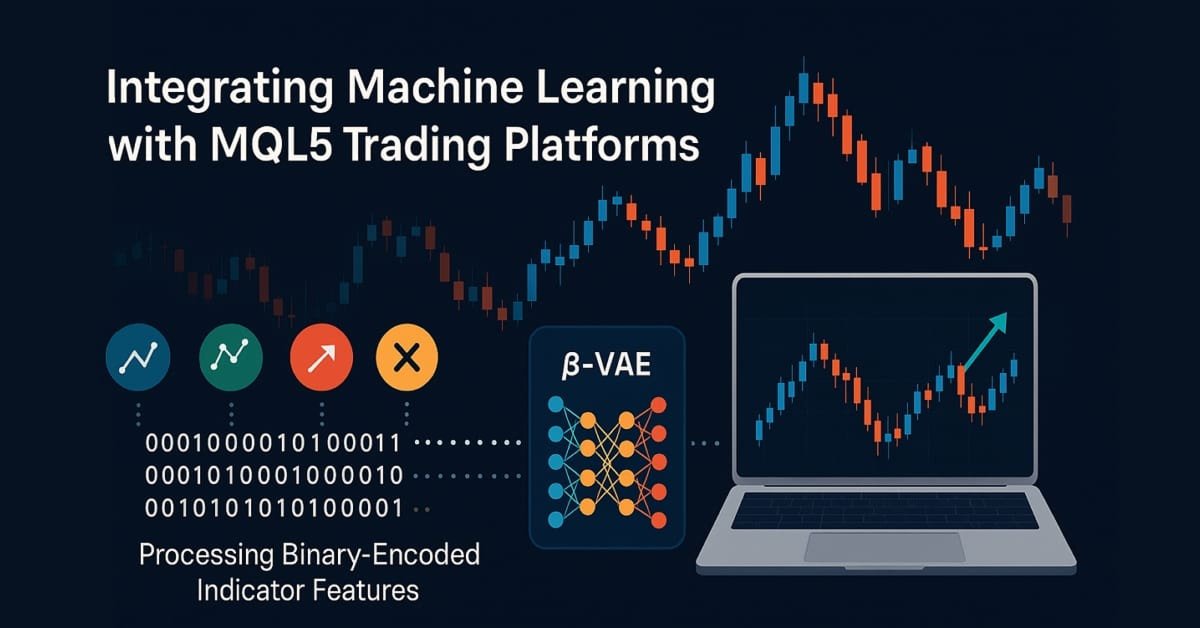
Among the available modern machine learning methods, Variational Autoencoders (VAEs) have gained attention for their ability to compress noisy, high-dimensional data into structured latent representations. Unlike a simple autoencoder, a β-VAE introduces a controlled penalty that encourages its hidden layer to capture disentangled, meaningful features rather than memorizing raw inputs. In financial trading, this translates to extracting the essence of patterns from streams of technical indicators, and less susceptibility to noise.

But the key insight — and the subject of this article — is that VAEs become especially powerful when they operate on binary-encoded features. Instead of feeding in continuous indicator values or scaled pipelines, we define clear, event-driven conditions. Did the Ichimoku Tenkan-sen cross above the Kijun-sen?, we assign 1 if yes, or 0 if no; Did the closing price break below the cloud?, again 1 if yes, 0 if no; Did the ADX above 25, confirming a strong trend?, same thing.

We are working with patterns 0, 1, and 5 of this Indicator pairing, Ichimoku & ADX, and these may appear as follows on a chart.

Pattern-0

Bearish signal where price crosses below the Senkou span A, marking a breakout below Kumo cloud. This is backed by ADX reading at least 25.

Pattern-1

Bearish signal, where Tenkan-Sen crosses the Kijun-Sen from above to close below it, signaling a short term change in momentum, towards short. The ADX would  be at least 20.

Pattern-5

Bullish signal when price bounces off the Tenkan-Sen with the ADX being at least at the 25 threshold.

Our premise in implementing this, for this article, is that these binary encodings form compact vectors that express whether important patterns are present or absent at each moment in time. When passed through the VAE, they provide a much cleaner signal structure than some pipelines of normalized floats. In our testing here, this adjustment alone improved the training process and resulted in stronger signals during testing.

This article will walk through how to implement this system. We will combine the Ichimoku indicator with Wilder’s ADX, generate binary feature vectors, train a β-VAE on historical market data, and then export the trained model into an ONNX format for use inside MQL5. Finally, we will review the strategy tester results to show how binary encodings performed given our backdrop/ recent foray into continuous-value pipelines, explored recently.

The MQL5 Wizard

The MQL5 Wizard lets traders quickly assemble Expert Advisors from predefined blocks—signals, money management, exits, and trailing stops—without writing boilerplate code. One of the more important features to traders who are slightly further-along, is the insertion of custom signal classes into a wizard built Expert Advisor. For the uninitiated, a signal class is where you set the actual logic of which trades need to be opened, and when they should be closed. MetaQuotes does provide standard signals that include Moving Averages or the RSI, however, custom signals tend to expand the wizard’s power significantly. With a custom signal class, we can connect machine learning models, probabilistic-forecasts, or as in this case a beta-VAE, to any of the inbuilt, standard signal patterns as traders seek not just alpha, but volatility stabilized portfolios.

A key feature is the ability to insert custom signal classes. While built-in signals include MA or RSI, custom classes can integrate machine learning models, probabilistic forecasts, or a VAE. The Wizard handles order management and position sizing, while the custom logic provides adaptability, helping filter false signals and enabling more context-aware strategies.

Pipelines and Binary Inputs

In the article prior to the last, we considered how SCIKIT-LEARN style preprocessing pipelines could be of use in normalizing features of a model, prior to training as well as inference. The notion was straightforward, apply imputation, scaling, and transformation steps systematically, so that all indicator values fall within comparable ranges. Methods that included min-max scaling, standard-scaling, as well as robust-scaling were engaged to prepare Ichimoku and ADX-Wilder data prior to being fed to a model. However, as we saw, this approach had a pair of weaknesses when trading.

Firstly, there was a loss of signal clarity. The scaling of continuous values ended up smoothing the very conditions we wanted to emphasize or identify. For instance, a breakout above the Ichimoku cloud - a clear boolean/binary even - became diluted into a floating point difference after normalization. In essence, the model was being forced to re-learn what traders already knew was pretty obvious - the moment crossovers or breakouts occur.

Secondly, while training, we experienced poor-stability. The outputted continuous features tended to amplify noise. Market fluctuations that have no clear causality and are random, do not matter in practice, and yet they were given equal importance by the scaler transformers. This resulted in slower convergence when training and weaker inference once deployed in live testing.

The solution, it appears, was to change our perspective. Instead of requiring our model(s) to interpret the size of differences, we  sought to mark whether certain conditions are present or not. This is the gist of converting indicator patterns into boolean or binary inputs. For instance, if Tenkan-Sen crossed the Kijun-Sen with the ADX above 20 we would mark this as an affirmative bullish signal for a particular pattern, and we would assign it 1. Anything else would get a 0. Likewise, if the closing price broke below Senkou-Span A, while the ADX did hold above the 25 we would assign a definitive 1, with any other indication receiving a 0 as far as this specific pattern is concerned.

These boolean encodings were represented in a clean vector of pattern-on/pattern-off signals, for every price-bar. So, rather than using pipelines to produce scaled-floats our get-features function from the VAE python code, below, directly assembles the boolean vectors

def GetFeatures(functions, *args, **kwargs) -> np.ndarray:
    features_per_func = []
    n_rows = None
    for f in functions:
        out = f(*args, **kwargs)
        a = np.asarray(out)
        if a.ndim == 1:
            row = SetRow(a)
            block = row
        elif a.ndim == 2:
            rows = [SetRow(a[i, :]) for i in range(a.shape[0])]
            block = np.concatenate(rows, axis=0)
        else:
            raise ValueError("Feature function returned array with ndim "+str(a.ndim))
        if n_rows is None:
            n_rows = block.shape[0]
        elif block.shape[0] != n_rows:
            raise ValueError("Inconsistent number of rows across feature functions.")
        features_per_func.append(block)
    return np.concatenate(features_per_func, axis=1)


def GetStates(df):
    diffs = df['close'].diff()
    df['states'] = np.select(
        condlist=[diffs > 0, diffs < 0],
        choicelist=[1.0, -1.0],
        default=0.0
    )
    return df[['states']]

It is noteworthy, that unlike in past articles where we chose to not combine signal patterns, and kept each distinct such that we ended up with a model for each signal pattern, in this article we are combining the 3 studied signal patterns into one. Just the three, not the original 10. This means we develop and test only one model.

The impact of this, it appears, was immediate. The VAE no longer has to figure out which portions of the numeric scale correspond to meaningful events and which are twat. Instead, it works with on/off flags that are arguably better aligned with trader intuition. When back testing, this design change is set up for better stability, as well as post-test live performance. In a market environment such as this where a significant retracement in equities is on the cards, and this is bound to entail a lot of volatility, a binary representation is bound to better model a distinction between noise and valid continuation signals. 

So, our step away from pipelines and embrace of binary-event-coding, not only simplifies the actual preprocessing, but it also gives our model, the beta-VAE, the sort of input it was designed to compress and represent effectively.

The Beta Variational Autoencoder

Once we have the boolean feature vectors defined, our next move is to pass them to a model. Python’s ability to handle this and similar steps in batches is part of the reason why it is very efficient when training. Add to this, the use of tensors when back propagating does bring extra buffering/ storage for registered gradients with each forward pass. Our VAE model is designed to be capable of learning compact representations of recurring market structures. This is a key selling point for the beta-VAE.

A standard autoencoder does compress/zip its inputs into a layer that is hidden. This is often also referred to as the latent space. Once this is done, it reconstructs them, back to their original form. A ‘variational’ autoencoder, takes this a notch further by making the latent space probabilistic. This hidden layer gets modelled as a distribution instead of fixed points. The encoder, therefore, produces both a mean and a variance when training. It is from this distribution that a random sample is selected in what is also referred to re-parameterization.

The beta-VAE, then, picks up where the regular VAE above leaves-off by adding one more twist. It multiplies the KL divergence term in the loss function by a factor beta. The effect of this, is that it strengthens regularization, which in turn encourages the model to learn disentangled meaningful features instead of memorizing inputs. In trading, this is vital because it enables the latent space to better code key patterns, such as a cloud breakout or even a trend continuation, instead of being pointlessly ‘democratic’ with noise.

Our model, is broken into the following key components:

• Encoder: This takes the boolean input feature vector, and passes it on through the dense layers. The output of this, being a distribution representation, is a mean (z_mean) and the logarithm of the variance (z_logvar).
• Re-Parameterization: This samples z from the latent Gaussian distribution. In this case, z is the ‘implied output’ of the input features, and as already mentioned and as is well known, encoders train to build a pair of weight matrices between the visible and hidden to allow for the ‘standard’ encoding of any pertinent input data.
• Decoder: This then tries to reconstruct the original input boolean vector from z. The effect of this is to force the latent space to focus, or capture the core structure of the earlier inputs. 
• Latent - y head: Finally, we have a supervised prediction head mapping z to an estimated value, y. In our case, this is amounts to a forecast trend in price action as either bullish or bearish or flat.

The loss function we engage for this VAE brings together three loss values. First, the reconstruction loss as measured using the binary cross entropy between the reconstructed outputs and the prior binary input features. Secondly, we have the KL divergence that penalizes deviation of latent distributions from the standard Gaussian prior. This is the case where the beta-multiplier becomes applicable. Thirdly, we have the head, supervised loss. This, for our purposes, is simply a mean squared error or MSE term between the predicted y final output and the actual y output. 

Our VAE input layer is special in that along with the typical indicator input features, we add a dimension for the expected output. When inputting, we assign this dim a neutral value of 0.5. After a cycle to the latent space and back to the input, the y output would be the missing next price action that follows or is paired with the 6 input features earlier provided. This means that it operates in two modes, where each mode provides a different output. Below is the listing to the beta-VAE implementation in Python;

# ----------------------------- β-VAE (inference simplified to VAE-only) -----------------------------
class BetaVAEUnsupervised(nn.Module):
    """
    Encoder: features -> (mu, logvar)
    Decoder: z -> x_hat
    **Inference (now VAE-only):** latent z is mapped to y via an internal head.
    All former infer modes (ridge/knn/kernel/lwlr/mlp) are bypassed.
    """
    def __init__(self, feature_dim, latent_dim, k_neighbors=5, beta=4.0, recon='bce',
                 infer_mode='vae', ridge_alpha=1e-2, kernel_bandwidth=1.0):
        super().__init__()
        self.latent_dim = latent_dim
        self.k_neighbors = k_neighbors
        self.beta = beta
        self.recon = recon
        self.infer_mode = 'vae'  # force VAE-only
        self.ridge_alpha = float(ridge_alpha)
        self.kernel_bandwidth = float(kernel_bandwidth)

        # Encoder
        self.feature_encoder = nn.Sequential(
            nn.Linear(feature_dim, 256), nn.ReLU(),
            nn.Linear(256, 128), nn.ReLU(),
            nn.Linear(128, latent_dim * 2)
        )
        # Decoder
        self.decoder = nn.Sequential(
            nn.Linear(latent_dim, 128), nn.ReLU(),
            nn.Linear(128, 256), nn.ReLU(),
            nn.Linear(256, feature_dim)
        )
        # New: latent→y head (supervised head trained with MSE)
        self.y_head = nn.Sequential(
            nn.Linear(latent_dim, 128), nn.ReLU(),
            nn.Linear(128, 1)
        )

    def encode(self, features):
        h = self.feature_encoder(features)
        z_mean, z_logvar = torch.chunk(h, 2, dim=1)
        return z_mean, z_logvar

    def reparameterize(self, mean, logvar):
        std = torch.exp(0.5 * logvar)
        eps = torch.randn_like(std)
        return mean + eps * std

    def decode(self, z):
        return self.decoder(z)

    def predict_from_latent(self, z):
        # VAE-only mapping
        return self.y_head(z)

    def forward(self, features, y=None):
        mu, logvar = self.encode(features)
        z = self.reparameterize(mu, logvar)
        x_logits = self.decode(z)
        y_hat = self.predict_from_latent(z)
        if y is not None:
            return {'z': z, 'z_mean': mu, 'z_logvar': logvar, 'x_logits': x_logits, 'y_hat': y_hat}
        else:
            return {'y': y_hat}

# Reconstruction + KL
def beta_vae_loss(features, x_logits, mu, logvar, beta=4.0, recon='bce'):
    if recon == 'bce':
        recon_loss = F.binary_cross_entropy_with_logits(x_logits, features, reduction='sum') / features.size(0)
    else:
        recon_loss = F.mse_loss(torch.sigmoid(x_logits), features, reduction='mean') * features.size(1)
    kl = -0.5 * torch.sum(1 + logvar - mu.pow(2) - logvar.exp()) / features.size(0)
    loss = recon_loss + beta * kl
    return loss, recon_loss.detach(), kl.detach()

In the forward pass function, we can either receive the y, next price action value, or this value plus the distribution vector that captures the z mean and variance. For our purposes when exporting to ONNX, since training is done, we always only output just the y value which points to the next price action where anything above 0.5f is bullish and anything below is bearish. 

Returning to the combined three loss values, merging them together when training, does encourage the model to both compress binary features while remaining predictive of price direction. The training procedure is executed with Adam Optimization across several epochs. For our model, we used 50 epochs. For each training step, though: features get encoded where the latent variables of the mean and variance get sampled for z; the decoder reconstructs the original features; the latent layer outputs to a head to forecast the next market state; a loss is computed in the event that a y input was provided and that we are therefore in training; and finally backpropagation updates weights not just for the VAE but also the head.

The loop of training that we perform uses a bootstrap that allows us to efficiently iterate over a data set while also printing epoch by epoch loss summaries. The prints allow monitoring on how the VAE is capable at drawing a balance between compression and disentanglement, as well as its predictive accuracy on the next states as provided by the head.

Exporting to MQL5

As regular readers know, training in Python is half the journey. To use models developed in this non-MQL5 language, within an Expert Advisor assembled by the wizard, we need a bridge. This, as already demonstrated in past articles, is ONNX, an abbreviation for Open Neural Network Exchange. This ‘bridge’ gives us a standardized format for representing models that are trained in Python to be used in a variety of other platforms, beyond MetaTrader. When, we export it to MQL5, however, this file which can range in size from a few hundred kilobytes all the way up to 128mb, as per my last testing with MQL5; can be loaded by various runtimes. This includes those accessible through its sandbox file system or via resource compilation. The bottom line here is we efficiently train advanced models with PyTorch, validate them in Python, and then deploy them for use with Expert Advisors, without re-writing any model logic. This process is chiefly handled by ‘export_onnx_y’ function. This is listed as follows:

import torch
import torch.nn as nn
import onnx
import onnxruntime as ort

def export_onnx_y(model: nn.Module, feature_dim: int, output_path: str,
                  opset: int = 14):
    """
    Export the VAE so that ONNX takes ONLY `features` and returns the inferred y.
    No latent (z, mu, logvar) are exported. No `y` input is used.
    """
    model.eval()

    # Wrapper that returns a plain tensor (y_hat), suitable for ONNX export
    class _YOnly(nn.Module):
        def __init__(self, m: nn.Module):
            super().__init__()
            self.m = m
        def forward(self, features: torch.Tensor) -> torch.Tensor:
            mu, logvar = self.m.encode(features)
            z = self.m.reparameterize(mu, logvar)
            y_hat = self.m.predict_from_latent(z)
            return y_hat  # shape: [N, 1]

    wrapped = _YOnly(model)

    dummy_features = torch.randn(1, feature_dim, dtype=torch.float32)

    torch.onnx.export(
        wrapped,
        dummy_features,
        output_path,
        input_names=["features"],
        output_names=["y_hat"],
        dynamic_axes={
            "features": {0: "batch_size"},
            "y_hat":    {0: "batch_size"},
        },
        opset_version=opset,
        do_constant_folding=True,
    )

    # Validate and print IO for sanity
    onnx_model = onnx.load(output_path)
    onnx.checker.check_model(onnx_model)
    print(f"ONNX model '{output_path}' exported and validated (features -> y_hat).")

    sess = ort.InferenceSession(output_path)
    for i in sess.get_inputs():
        print(f"input:  {i.name}, shape={i.shape}, type={i.type}")
    for o in sess.get_outputs():
        print(f"output: {o.name}, shape={o.shape}, type={o.type}")

The export function above constructs a clean production-ready ONNX head. This is ready for forward passing to map precomputed features from our two indicators to then output a solo y value without any extra debug outputs or inputs. In doing so, it starts by switching the PyTorch VAE into eval-mode in order to freeze the dropout/ batch normalization behavior. Once this is addressed, it runs encode features to get the mean and variance, followed by sampling a latent vector z, through the afore mentioned re-parameterization-trick. This then feeds z through the model’s function of predict-from-latent head, following which it returns the y value in the shape [batch, 1]. This wrapper is instantiated around the trained model to ensure the exported graph includes the minimum forward pass features.

Just one dummy input tensor of shape [1, 6] gets created to help trace the graph. The torch.onnx.export module then gets invoked with explicit naming and with dynamic axes on the batch dimension so that the exported model gets to accept any batch size. The opset parameter is defaulted to 14 and also constant folding is enabled in order to make the graph simpler to interpret. 

Within Python, even after exporting, we need to instantly validate the file by re-importing and also performing checks on the size on input and output layers. We do this by loading the file with the onnx.load module, we then perform a check using onnx.checker.check_model to see if it is valid and open in a suitable inference session. We print off the discovered input and output layer signatures, which are important inputs when we get to MetaTrader. Our chosen export model simplifies the VAE model to almost look like a supervised learning network, however as already argued above, it is a VAE that automatically inputs the missing y input with a neutral zero value, performs a complete cycle from input to hidden and back, and then infers the missing value based on the trained weights of the VAE.

Once exported, the ONNX file, needs to be instantly validated within MQL5. Rather than refer to an ONNX file in the sandbox, we are electing as we’ve been doing in the past to import this file as a resource. This option has implications though on how large an exported model can be. It used to be that the limit of a resource file was about 256mb, but lately this appears to have reduced to half that value and settling at around 128mb. I am yet to confirm, this, but none-resource ONNX files, that reside in a sandbox, may not face similar limitations. These limitations could be in place, especially for traders who count on using the MQL5 VPS.

Running Inference from partial Features to Forecasts

The process of training a model is always just a single step; using it as anticipated in live trading is often a different proposition. Once the beta-VAE is exported to ONNX, it gets called, as a resource in our case, to make forecasts. Within Python, though, we test how this inference will work in MQL5, by running some synthetic binary with the infer_example function. This can help indicate if preset long or short indicator readings will actually get interpreted as expected.

# ----------------------------- Inference demo (updated) -----------------------------
def infer_example(model, dataloader=None, num_examples=5, prob_one_in_pair=0.6, seed=None, partial_rows=None):
    """
    If partial_rows is provided, we zero-fill missing inputs and run a full VAE cycle
    to produce y that pairs with that incomplete input.
    Otherwise, we keep the previous synthetic-pairs demo using the dataloader.
    """
    model.eval()
    with torch.no_grad():
        if partial_rows is not None:
            device = next(model.parameters()).device
            X = _zero_fill_rows(partial_rows, feature_dim, device)
            preds = model(X)
            print("Inference with partial inputs (zero-filled):")
            for i in range(X.size(0)):
                yhat = float(preds['y'][i].item())
                print(f"X[{i}] first 8: {X[i, :8].tolist()} -> y_hat={yhat:.6f}")
            return
        # ----- legacy synthetic example (kept) -----
        if dataloader is None:
            raise ValueError("dataloader required when partial_rows is None")
        batch = next(iter(dataloader))
        N = min(num_examples, batch["features"].shape[0])
        feat_dim = batch["features"].shape[1]
        assert feat_dim >= 6 and feat_dim % 2 == 0, "feature_dim must be even and >= 6"
        pairs = 3
        device = next(model.parameters()).device
        if seed is not None:
            torch.manual_seed(seed)
        X = torch.zeros((N, feat_dim), device=device)
        any_one = torch.bernoulli(torch.full((N, pairs), float(prob_one_in_pair), device=device)).bool()
        side = torch.bernoulli(torch.full((N, pairs), 0.5, device=device)).long()
        row_idx = torch.arange(N, device=device).unsqueeze(1).expand(N, pairs)
        base = (torch.arange(pairs, device=device).unsqueeze(0).expand(N, pairs) * 2)
        col_idx = base + side
        sel_rows = row_idx[any_one]; sel_cols = col_idx[any_one]
        X[sel_rows, sel_cols] = 1.0
        preds = model(X)
        print(" Example Inference (3 exclusive pairs):")
        for i in range(N):
            yhat = float(preds['y'][i].item())
            print(f"X[{i}]={X[i, :6].int().tolist()}{'...' if feat_dim > 6 else ''} -> ŷ={yhat:.5f}")

Markets rarely present a full vector of clean signals at all the price bars. Often the case is that the Tenkan-Kijun cross over is evident, however the cloud breakout is missing. To better simulate this, our inference example supports partial inputs, where zero being the default for missing values. Also, noteworthy is that our simulation here takes care to ensure both long and short conditions are not simultaneously inputted into the model, as this is not possible based on how the indicator features are defined.

Strategy Tester Results

The proof is always in the eating of the pudding, as they say and whereas strictly speaking for traders this would involve aspects of trade account management that encompass planning withdrawals, which MetaTrader can simulate, for our purposes we will dwell on the profitability of the model when tested in MQL5. After we trained the beta-VAE on boolean encoded features from indicator readings of EUR USD, on the 4-hour time frame, from 2023.07.01 to 2024.07.01, we exported this for forward walking from 2024.07.01 to 2025.07.01 in MetaTrader. The forward test results, while subject to the usual disclaimer, were better than what we had in the last article where we engaged pipelines in a reinforcement learning model. 

There are many moving parts here, the different learning types (inference vs reinforcement), varying model types (beta-VAE vs TD3), and the fact that our test window is restricted to just the one year. Also, more elaborate techniques of regularization were not engaged to ensure the test window has a balanced target data of roughly equal count of long price action states and short price action. This is why our reports all indicate only long trades. These and other more elaborate points are not properly addressed here, however the MQL code is attached and the overall approach in Python is outlined, so traders can take this further for more development.

With that said, since we are almost on an even comparison footing with the last article’s testing environment, it could be insightful for us to compare binary feature input model performance versus the pipeline input model results. When we relied on the SCIKIT-LEARN style pipelines, the model in play was receiving continuos values from the gaps and difference in the Ichimoku and the ADX. While the training results were promising with declining losses, the forward walk indicated the contrary. The equity curve results, going forward, were also unstable with poor risk-reward ratio. This same problem does apply in our better results with binary input vectors, partly because we are not using a stop-loss.

We also had a lot of false positive signals during choppy rebounds with the 3 tests on the 3 patterns 0, 1, and 5. These were all independent, unlike in this article, where we have unified their indicator readings as input to a single VAE model. That is also another major distinction from our last article.

The binary encoding approach by contrast appears to present clearer results with consistently upward equity, with the execution of very few trades that were all accurate. This is across the same test window. While this one year test window is limited, and we are running a trade setup without proper stop management, this like for like comparison between pipeline scaling model and boolean inputs does point to the strengths of the latter. It could be we are reaping the benefits of ‘stripping away noise’ in the form of floating/continuous inputs when we use yes/no data instead.

Conclusion

In this article we have shown, as usual, how the wizard can be extended beyond the regular inbuilt signal library by incorporating inference learning - in this case, a beta Variational Autoencoder that is trained on boolean indicator patterns. By encoding Ichimoku and ADX Wilder conditions in a binary yes/no vectors, it appears we reduced noise present in market data, unlike when we were using pipeline transformers where it seems we only amplified this. From our limited time window of just 2 years, one training and one testing, we were able to get a stable training process, cleaner latent representations, as well as some improved performance in the Strategy Tester. As usual, testing in wider window periods and on broker real tick data is always necessary before more definitive conclusions can be drawn.

name	description
81b.mq5	Wizard Assembled Expert, whose header lists referenced files
SignalWZ_81b.mqh	Custom Signal Class file that incorporates Inference Learning
81_.onnx	ONNX Exported model. Imported as a resource