Using PatchTST Machine Learning Algorithm for Predicting Next 24 Hours of Price Action

Introduction

I first encountered an algorithm called PatchTST when I started to dig into the AI advancements associated with time series predictions on Huggingface.co. As anyone who has worked with large language models (LLMs) would know, the invention of transformers has been a game changer for developing tools for natural language, image, and video processing. But what about time series? Is it something that's just left behind? Or is most of the research simply behind closed doors? It turns out there are many newer models that apply transformers successfully for predicting time series. In this article, we will look at one such implementation.

What's impressive about PatchTST is how quick it is to train a model and how easy it is to use the trained model with MQL. I admit openly that I am new to the concept of neural networks. But going through this process and tackling the implementation of PatchTST outlined in this article for MQL5, I felt like I took a giant leap forward in my learning and understanding of how these complex neural networks are developed, troubleshot, trained, and used. It is like taking a child, who is barely learning to walk, and putting him on a professional soccer team, expecting him to score the winning goal in the World Cup final. 

PatchTST Overview

After discovering PatchTST, I started to look into the paper that explains its design: "A Time Series is Worth 64 Words: Long-term Forecasting with Transformers". The title was interesting. As I started to read more into the paper, I thought wow this looks like an fascinating structure - it has many elements that I have always wanted to learn about. So naturally, I wanted to try it out and see how the predictions work. Here is what made me even more interested in this algorithm:

• You can predict open, high, low, and close using PatchTST. With PatchTST, I felt that you couldfeed it the entire data as it comes - open, high, low, close, and even volume. You can expect it to find the patterns in the data because all the data is converted to something called "patches". More on what patches are a little later in this article. For now, it is just important to know that patches are appealing and help make predictions better.
• Minimal data-preprocessing requirements with PatchTST. As I started to dig into the algorithm further, I realized that the authors use something called "RevIn", which is reverse instance normalization. RevIn comes from a paper titled: "REVERSIBLE INSTANCE NORMALIZATION FOR ACCURATE TIME-SERIES FORECASTING AGAINST DISTRIBUTION SHIFT". RevIn attempts to tackle the problem of distribution shift in time-series forecasting. As algorithmic traders, we are all too familiar with the feeling when our trained EA no longer seems to predict the market, and we are forced to re-optimize and update our parameters. Consider RevIn to be a way to do the same thing. 
  
  
• This is method basically takes the data passed into it and normalizes it using the following formula:

x = (x - mean) / std

Then, when the model has to make a prediction, it denormalizes the data using the opposite property:

x = x * std + mean

RevIn also has another property called affine_bias. In the simplest possible terms, this is a learnable parameter that takes care of the skewness, kurtosis etc. that may be present in the dataset. 

x = x * affine_weight + affine_bias

The structure of PatchTST can be summarized as follows: 

Input Data -> RevIn -> Series Decomposition -> Trend Component -> PatchTST Backbone -> TSTiEncoder -> Flatten_Head -> Trend Forecaster -> Residual Component -> Add Trend and Residual -> Final Forecast

We understand that our data will be pulled using MT5. We have also discussed how RevIn works.

Here is how PatchTST works: say you pull 80,000 bars of EURUSD data for the H1 timeframe. That is just around 13 years’ worth of data. With PatchTST, you segment the data into something called “patches”. As an analogy, think of patches as being similar to how Vision Transformers (ViTs) work for images but adapted for time series data. So, for example, if the patch length is 16, then each patch would contain 16 consecutive price values. This is like looking at small chunks of the time series at a time, which helps the model to focus on local patterns before considering the global pattern.

Next, the patches include positional encoding to preserve the sequence order, which assists the model in remembering the position of each patch in the sequence.

The transformer passes the normalized and encoded patches through a stack of encoder layers. Each encoder layer contains a multi-head attention layer and a feed-forward layer. The multi-head attention layer allows the model to attend to different parts of the input sequence, while the feed-forward layer allows the model to learn complex non-linear transformations of the data.

Lastly, we have the trend and the residual components. The same patching, normalization, positional encoding, and transformer layers are applied to both the trend component and the residual component. Then, we add together the outputs of the trend and residual components to produce the final forecast.

PatchTST Official Repository Issues

The official repository for PatchTST can be found on GitHub at the following link: PatchTST (ICLR 2023). There are two different versions available - supervised and unsupervised. For this article, we will use the supervised learning approach. As we know, in order to use any model with MQL5, we need a way to convert it to ONNX format. However, the authors of PatchTST did not take this into account. I had to make the following modifications to their base code to make the model work with MQL5: 

Original Code: 

class PatchTST_backbone(nn.Module):
    def __init__(self, c_in:int, context_window:int, target_window:int, patch_len:int, stride:int, max_seq_len:Optional[int]=1024, 
                 n_layers:int=3, d_model=128, n_heads=16, d_k:Optional[int]=None, d_v:Optional[int]=None,
                 d_ff:int=256, norm:str='BatchNorm', attn_dropout:float=0., dropout:float=0., act:str="gelu", key_padding_mask:bool='auto',
                 padding_var:Optional[int]=None, attn_mask:Optional[Tensor]=None, res_attention:bool=True, pre_norm:bool=False,                          
                 store_attn:bool=False,
                 pe:str='zeros', learn_pe:bool=True, fc_dropout:float=0., head_dropout = 0, padding_patch = None,
                 pretrain_head:bool=False, head_type = 'flatten', individual = False, revin = True, affine = True, subtract_last = False,
                 verbose:bool=False, **kwargs):
        
        super().__init__()
        
        # RevIn
        self.revin = revin
        if self.revin: self.revin_layer = RevIN(c_in, affine=affine, subtract_last=subtract_last)
        
        # Patching
        self.patch_len = patch_len
        self.stride = stride
        self.padding_patch = padding_patch
        patch_num = int((context_window - patch_len)/stride + 1)
        if padding_patch == 'end': # can be modified to general case
            self.padding_patch_layer = nn.ReplicationPad1d((0, stride)) 
            patch_num += 1
        
        # Backbone 
        self.backbone = TSTiEncoder(c_in, patch_num=patch_num, patch_len=patch_len, max_seq_len=max_seq_len,
                                n_layers=n_layers, d_model=d_model, n_heads=n_heads, d_k=d_k, d_v=d_v, d_ff=d_ff,
                                attn_dropout=attn_dropout, dropout=dropout, act=act, key_padding_mask=key_padding_mask, padding_var=padding_var,
                                attn_mask=attn_mask, res_attention=res_attention, pre_norm=pre_norm, store_attn=store_attn,
                                pe=pe, learn_pe=learn_pe, verbose=verbose, **kwargs)

        # Head
        self.head_nf = d_model * patch_num
        self.n_vars = c_in
        self.pretrain_head = pretrain_head
        self.head_type = head_type
        self.individual = individual

        if self.pretrain_head: 
            self.head = self.create_pretrain_head(self.head_nf, c_in, fc_dropout) # custom head passed as a partial func with all its kwargs
        elif head_type == 'flatten': 
            self.head = Flatten_Head(self.individual, self.n_vars, self.head_nf, target_window, head_dropout=head_dropout)
        
    
    def forward(self, z):                                                                   # z: [bs x nvars x seq_len]
        # norm
        if self.revin: 
            z = z.permute(0,2,1)
            z = self.revin_layer(z, 'norm')
            z = z.permute(0,2,1)
            
        # do patching
        if self.padding_patch == 'end':
            z = self.padding_patch_layer(z)
        z = z.unfold(dimension=-1, size=self.patch_len, step=self.stride)                   # z: [bs x nvars x patch_num x patch_len]
        z = z.permute(0,1,3,2)                                                              # z: [bs x nvars x patch_len x patch_num]
        
        # model
        z = self.backbone(z)                                                                # z: [bs x nvars x d_model x patch_num]
        z = self.head(z)                                                                    # z: [bs x nvars x target_window] 
        
        # denorm
        if self.revin: 
            z = z.permute(0,2,1)
            z = self.revin_layer(z, 'denorm')
            z = z.permute(0,2,1)
        return z

Code above is the main backbone. As you can see, the code uses a function called Unfold in the line: 

 z = z.unfold(dimension=-1, size=self.patch_len, step=self.stride)                   # z: [bs x nvars x patch_num x patch_len]

The conversion of Unfold is not supported by ONNX. You will receive an error like: 

Unsupported: ONNX export of operator Unfold, input size not accessible. Please feel free to request support or submit a pull request on PyTorch GitHub: https://github.com/pytorch/pytorch/issues

So I had to replace this section of the code with: 

# Manually unfold the input tensor
    batch_size, n_vars, seq_len = z.size()
    patches = []
    for i in range(0, seq_len - self.patch_len + 1, self.stride):
        patches.append(z[:, :, i:i+self.patch_len])

Note that the above replacement is a little less efficient because it uses a for loop for training a Neural Network. The inefficiencies can add up over many epochs and over large datasets. But this is necessary because otherwise, the model will simply fail to convert, and we will not be able to use it with MQL5. 

I specifically addressed this issue. Doing this took the longest. I then put everything together in a file called patchTST.py, which can be found in the zip file attached to this article. This is the file that we will be using for our model training. 

Requirements to Work with PatchTST in Python

In this section, I will give you the requirements for working with PatchTST in Python. These requirements can be summarized below: 

Create a virtual environment: 

python -m venv myenv

Activate the virtual environment (Windows)

.\myenv\Scripts\activate

Install the requirements.txt file included in the zip file attached to this article: 

pip install -r requirements.txt

Specifically, the requirements to run this project are: 

MetaTrader5
pandas
numpy
torch
plotly
datetime

Model Training Code Development Step-By-Step

For the following code, you can follow along with me using a Jupyter notebook that I have included in the zip file: PatchTST Step-By-Step.ipynb. We will summarize the steps below: 

1. Import Necessary Libraries: Importing the required libraries, including MetaTrader 5, Pandas, Numpy, Torch, and the PatchTST model.
   

   # Step 1: Import necessary libraries
   import MetaTrader5 as mt5
   import pandas as pd
   import numpy as np
   import torch
   from torch.utils.data import TensorDataset, DataLoader
   from patchTST import Model as PatchTST

2. Initialize and Fetch Data from MetaTrader 5: Function fetch_mt5_data initializes MT5, fetches the data for the given symbol, timeframe, and number of bars, then returns a data frame with the open, high, low, and close columns.
   

   # Step 2: Initialize and fetch data from MetaTrader 5
   def fetch_mt5_data(symbol, timeframe, bars):
       if not mt5.initialize():
           print("MT5 initialization failed")
           return None
   
       timeframe_dict = {
           'M1': mt5.TIMEFRAME_M1,
           'M5': mt5.TIMEFRAME_M5,
           'M15': mt5.TIMEFRAME_M15,
           'H1': mt5.TIMEFRAME_H1,
           'D1': mt5.TIMEFRAME_D1
       }
   
       rates = mt5.copy_rates_from_pos(symbol, timeframe_dict[timeframe], 0, bars)
       mt5.shutdown()
   
       df = pd.DataFrame(rates)
       df['time'] = pd.to_datetime(df['time'], unit='s')
       df.set_index('time', inplace=True)
       return df[['open', 'high', 'low', 'close']]
   
   # Fetch data
   data = fetch_mt5_data('EURUSD', 'H1', 80000)

3. Prepare Forecasting Data Using Sliding Window: The function prepare_forecasting_data creates the dataset using a sliding window approach, generating sequences of historical data (X) and the corresponding future data (y).
   

   # Step 3: Prepare forecasting data using sliding window
   def prepare_forecasting_data(data, seq_length, pred_length):
       X, y = [], []
       for i in range(len(data) - seq_length - pred_length):
           X.append(data.iloc[i:(i + seq_length)].values)
           y.append(data.iloc[(i + seq_length):(i + seq_length + pred_length)].values)
       return np.array(X), np.array(y)
   
   seq_length = 168  # 1 week of hourly data
   pred_length = 24  # Predict next 24 hours
   
   X, y = prepare_forecasting_data(data, seq_length, pred_length)

4. Split Data into Training and Testing Sets: Splitting the data into training and testing sets, with 80% for training and 20% for testing. 
   

   # Step 4: Split data into training and testing sets
   split = int(len(X) * 0.8)
   X_train, X_test = X[:split], X[split:]
   y_train, y_test = y[:split], y[split:]
   

5. Convert Data to PyTorch Tensors: Converting the NumPy arrays into PyTorch tensors, which are required for training with PyTorch. Sets a manual seed for torch, for reproducibility of results. 

   # Step 5: Convert data to PyTorch tensors
   X_train = torch.tensor(X_train, dtype=torch.float32)
   y_train = torch.tensor(y_train, dtype=torch.float32)
   X_test = torch.tensor(X_test, dtype=torch.float32)
   y_test = torch.tensor(y_test, dtype=torch.float32)
   
   torch.manual_seed(42)

6. Set Device for Computation: Setting the device to CUDA if available, otherwise using the CPU. This is essential for leveraging GPU acceleration during training, especially if it is available.
   

   # Step 6: Set device for computation
   device = torch.device("cuda" if torch.cuda.is_available() else "cpu")
   print(f"Using device: {device}")

7. Create Data Loader for Training Data: Creating a data loader to handle the batching and shuffling of the training data.
   

   # Step 7: Create DataLoader for training data
   train_dataset = TensorDataset(X_train, y_train)
   train_loader = DataLoader(train_dataset, batch_size=32, shuffle=True)

8. Define the Configuration Class for the Model: Defining a configuration class Config to store all the hyperparameters and settings required for the PatchTST model.
   

   # Step 8: Define the configuration class for the model
   class Config:
       def __init__(self):
           self.enc_in = 4  # Adjusted for 4 columns (open, high, low, close)
           self.seq_len = seq_length
           self.pred_len = pred_length
           self.e_layers = 3
           self.n_heads = 4
           self.d_model = 64
           self.d_ff = 256
           self.dropout = 0.1
           self.fc_dropout = 0.1
           self.head_dropout = 0.1
           self.individual = False
           self.patch_len = 24
           self.stride = 24
           self.padding_patch = True
           self.revin = True
           self.affine = False
           self.subtract_last = False
           self.decomposition = True
           self.kernel_size = 25
   
   configs = Config()

9. Initialize the PatchTST Model: Initializing the PatchTST model with the defined configuration and moving it to the selected device.
   

   # Step 9: Initialize the PatchTST model
   model = PatchTST(
       configs=configs,
       max_seq_len=1024,
       d_k=None,
       d_v=None,
       norm='BatchNorm',
       attn_dropout=0.1,
       act="gelu",
       key_padding_mask='auto',
       padding_var=None,
       attn_mask=None,
       res_attention=True,
       pre_norm=False,
       store_attn=False,
       pe='zeros',
       learn_pe=True,
       pretrain_head=False,
       head_type='flatten',
       verbose=False
   ).to(device)

10. Define Optimizer and Loss Function: Setting up the optimizer (Adam) and the loss function (Mean Squared Error) for training the model.
    

    # Step 10: Define optimizer and loss function
    optimizer = torch.optim.Adam(model.parameters(), lr=0.001)
    loss_fn = torch.nn.MSELoss()
    num_epochs = 100

11. Train the Model: Training the model over the specified number of epochs. For each batch of data, the model performs a forward pass, calculates the loss, performs a backward pass to compute gradients, and updates the model parameters.
    

    # Step 11: Train the model
    for epoch in range(num_epochs):
        model.train()
        total_loss = 0
        for batch_X, batch_y in train_loader:
            optimizer.zero_grad()
            batch_X = batch_X.to(device)
            batch_y = batch_y.to(device)
    
            outputs = model(batch_X)
            outputs = outputs[:, -pred_length:, :4]
    
            loss = loss_fn(outputs, batch_y)
    
            loss.backward()
            optimizer.step()
            total_loss += loss.item()
    
        print(f"Epoch {epoch+1}/{num_epochs}, Loss: {total_loss/len(train_loader):.10f}")

12. Save the Model in PyTorch Format: Saving the trained model's state dictionary to a file. We can use this file to make predictions directly in python. 
    

    # Step 12: Save the model in PyTorch format
    torch.save(model.state_dict(), 'patchtst_model.pth')

13. Prepare a Dummy Input for ONNX Export: Creating a dummy input tensor to use for exporting the model to ONNX format. 
    

    # Step 13: Prepare a dummy input for ONNX export
    dummy_input = torch.randn(1, seq_length, 4).to(device)

14. Export the Model to ONNX Format: Exporting the trained model to the ONNX format. We will need this file to make predictions with MQL5. 
    

    # Step 14: Export the model to ONNX format
    torch.onnx.export(model, dummy_input, "patchtst_model.onnx",
                      opset_version=13,
                      input_names=['input'],
                      output_names=['output'],
                      dynamic_axes={'input': {0: 'batch_size'},
                                    'output': {0: 'batch_size'}})
    
    print("Model trained and saved in PyTorch and ONNX formats.")

Model Training Results

Here are the results I obtained from training the model. 

Epoch 1/100, Loss: 0.0000283705
Epoch 2/100, Loss: 0.0000263274
Epoch 3/100, Loss: 0.0000256321
Epoch 4/100, Loss: 0.0000252389
Epoch 5/100, Loss: 0.0000249340
Epoch 6/100, Loss: 0.0000246715
Epoch 7/100, Loss: 0.0000244293
Epoch 8/100, Loss: 0.0000241942
Epoch 9/100, Loss: 0.0000240157
Epoch 10/100, Loss: 0.0000236776
Epoch 11/100, Loss: 0.0000233954
Epoch 12/100, Loss: 0.0000230437
Epoch 13/100, Loss: 0.0000226635
Epoch 14/100, Loss: 0.0000221875
Epoch 15/100, Loss: 0.0000216960
Epoch 16/100, Loss: 0.0000213242
Epoch 17/100, Loss: 0.0000208693
Epoch 18/100, Loss: 0.0000204956
Epoch 19/100, Loss: 0.0000200573
Epoch 20/100, Loss: 0.0000197222
Epoch 21/100, Loss: 0.0000193516
Epoch 22/100, Loss: 0.0000189223
Epoch 23/100, Loss: 0.0000186635
Epoch 24/100, Loss: 0.0000184025
Epoch 25/100, Loss: 0.0000180468
Epoch 26/100, Loss: 0.0000177854
Epoch 27/100, Loss: 0.0000174621
Epoch 28/100, Loss: 0.0000173247
Epoch 29/100, Loss: 0.0000170032
Epoch 30/100, Loss: 0.0000168594
Epoch 31/100, Loss: 0.0000166609
Epoch 32/100, Loss: 0.0000164818
Epoch 33/100, Loss: 0.0000162424
Epoch 34/100, Loss: 0.0000161265
Epoch 35/100, Loss: 0.0000159775
Epoch 36/100, Loss: 0.0000158510
Epoch 37/100, Loss: 0.0000156571
Epoch 38/100, Loss: 0.0000155327
Epoch 39/100, Loss: 0.0000154742
Epoch 40/100, Loss: 0.0000152778
Epoch 41/100, Loss: 0.0000151757
Epoch 42/100, Loss: 0.0000151083
Epoch 43/100, Loss: 0.0000150182
Epoch 44/100, Loss: 0.0000149140
Epoch 45/100, Loss: 0.0000148057
Epoch 46/100, Loss: 0.0000147672
Epoch 47/100, Loss: 0.0000146499
Epoch 48/100, Loss: 0.0000145281
Epoch 49/100, Loss: 0.0000145298
Epoch 50/100, Loss: 0.0000144795
Epoch 51/100, Loss: 0.0000143969
Epoch 52/100, Loss: 0.0000142840
Epoch 53/100, Loss: 0.0000142294
Epoch 54/100, Loss: 0.0000142159
Epoch 55/100, Loss: 0.0000140837
Epoch 56/100, Loss: 0.0000140005
Epoch 57/100, Loss: 0.0000139986
Epoch 58/100, Loss: 0.0000139122
Epoch 59/100, Loss: 0.0000139010
Epoch 60/100, Loss: 0.0000138351
Epoch 61/100, Loss: 0.0000138050
Epoch 62/100, Loss: 0.0000137636
Epoch 63/100, Loss: 0.0000136853
Epoch 64/100, Loss: 0.0000136191
Epoch 65/100, Loss: 0.0000136272
Epoch 66/100, Loss: 0.0000135552
Epoch 67/100, Loss: 0.0000135439
Epoch 68/100, Loss: 0.0000135200
Epoch 69/100, Loss: 0.0000134461
Epoch 70/100, Loss: 0.0000133950
Epoch 71/100, Loss: 0.0000133979
Epoch 72/100, Loss: 0.0000133059
Epoch 73/100, Loss: 0.0000133242
Epoch 74/100, Loss: 0.0000132816
Epoch 75/100, Loss: 0.0000132145
Epoch 76/100, Loss: 0.0000132803
Epoch 77/100, Loss: 0.0000131212
Epoch 78/100, Loss: 0.0000131809
Epoch 79/100, Loss: 0.0000131538
Epoch 80/100, Loss: 0.0000130786
Epoch 81/100, Loss: 0.0000130651
Epoch 82/100, Loss: 0.0000130255
Epoch 83/100, Loss: 0.0000129917
Epoch 84/100, Loss: 0.0000129804
Epoch 85/100, Loss: 0.0000130086
Epoch 86/100, Loss: 0.0000130156
Epoch 87/100, Loss: 0.0000129557
Epoch 88/100, Loss: 0.0000129013
Epoch 89/100, Loss: 0.0000129018
Epoch 90/100, Loss: 0.0000128864
Epoch 91/100, Loss: 0.0000128663
Epoch 92/100, Loss: 0.0000128411
Epoch 93/100, Loss: 0.0000128514
Epoch 94/100, Loss: 0.0000127915
Epoch 95/100, Loss: 0.0000127778
Epoch 96/100, Loss: 0.0000127787
Epoch 97/100, Loss: 0.0000127623
Epoch 98/100, Loss: 0.0000127452
Epoch 99/100, Loss: 0.0000127141
Epoch 100/100, Loss: 0.0000127229

The results can be visualized as follows: 

We also get the following output without any errors and warnings, indicating that our model has successfully been converted to ONNX format. 

Model trained and saved in PyTorch and ONNX formats.

Generating Predictions using Python Step-By-Step

Now let us look at the prediction code: 

1. Step 1. Import Required Libraries: we start by importing all the necessary libraries.
   

   # Import required libraries
   import MetaTrader5 as mt5
   import pandas as pd
   import numpy as np
   import torch
   from datetime import datetime, timedelta
   import plotly.graph_objects as go
   from plotly.subplots import make_subplots
   from patchTST import Model as PatchTST

2. Step 2. Fetch Data from Metatrader 5:  we define a function to fetch data from MetaTrader 5 and convert it into a DataFrame. We fetch 168 prior bars because that is what is required to get a prediction with our model. 
   

   # Function to fetch data from MetaTrader 5
   def fetch_mt5_data(symbol, timeframe, bars):
       if not mt5.initialize():
           print("MT5 initialization failed")
           return None
   
       timeframe_dict = {
           'M1': mt5.TIMEFRAME_M1,
           'M5': mt5.TIMEFRAME_M5,
           'M15': mt5.TIMEFRAME_M15,
           'H1': mt5.TIMEFRAME_H1,
           'D1': mt5.TIMEFRAME_D1
       }
   
       rates = mt5.copy_rates_from_pos(symbol, timeframe_dict[timeframe], 0, bars)
       mt5.shutdown()
   
       df = pd.DataFrame(rates)
       df['time'] = pd.to_datetime(df['time'], unit='s')
       df.set_index('time', inplace=True)
       return df[['open', 'high', 'low', 'close']]
   
   # Fetch the latest week of data
   historical_data = fetch_mt5_data('EURUSD', 'H1', 168)

3. Step 3. Prepare Input Data: we define a function to prepare the input data for the model by taking the last seq_length rows of data. When pulling data, we only require the last 168 hours of 1h data to make predictions for the next 24 hours. This is because that is how we trained the model. 
   

   # Function to prepare input data
   def prepare_input_data(data, seq_length):
       X = []
       X.append(data.iloc[-seq_length:].values)
       return np.array(X)
   
   # Prepare the input data
   seq_length = 168  # 1 week of hourly data
   input_data = prepare_input_data(historical_data, seq_length)
   

4. Step 4. Define Configuration: we define a configuration class to set up the parameters for the model. These settings are the same as the ones we use for training the model. 
   

   # Define the configuration class
   class Config:
       def __init__(self):
           self.enc_in = 4  # Adjusted for 4 columns (open, high, low, close)
           self.seq_len = seq_length
           self.pred_len = 24  # Predict next 24 hours
           self.e_layers = 3
           self.n_heads = 4
           self.d_model = 64
           self.d_ff = 256
           self.dropout = 0.1
           self.fc_dropout = 0.1
           self.head_dropout = 0.1
           self.individual = False
           self.patch_len = 24
           self.stride = 24
           self.padding_patch = True
           self.revin = True
           self.affine = False
           self.subtract_last = False
           self.decomposition = True
           self.kernel_size = 25
   
   # Initialize the configuration
   config = Config()

5. Step 5. Load The Trained Model: we define a function to load the trained PatchTST model. These are the same settings as we used for training the model. 
   

   # Function to load the trained model
   def load_model(model_path, config):
       model = PatchTST(
           configs=config,
           max_seq_len=1024,
           d_k=None,
           d_v=None,
           norm='BatchNorm',
           attn_dropout=0.1,
           act="gelu",
           key_padding_mask='auto',
           padding_var=None,
           attn_mask=None,
           res_attention=True,
           pre_norm=False,
           store_attn=False,
           pe='zeros',
           learn_pe=True,
           pretrain_head=False,
           head_type='flatten',
           verbose=False
       )
       model.load_state_dict(torch.load(model_path))
       model.eval()
       return model
   
   # Load the trained model
   model_path = 'patchtst_model.pth'
   device = torch.device("cuda" if torch.cuda.is_available() else "cpu")
   model = load_model(model_path, config).to(device)
   

6. Step 6. Make Predictions: we define a function to make predictions using the loaded model and input data.
   

   # Function to make predictions
   def predict(model, input_data, device):
       with torch.no_grad():
           input_data = torch.tensor(input_data, dtype=torch.float32).to(device)
           output = model(input_data)
       return output.cpu().numpy()
   
   # Make predictions
   predictions = predict(model, input_data, device)
   

7. Step 7. Post-Processing and Visualization: we process the predictions, create a data frame, and visualize the historical and predicted data using Plotly.
   

   # Ensure predictions have the correct shape
   if predictions.shape[2] != 4:
       predictions = predictions[:, :, :4]  # Adjust based on actual number of columns required
   
   # Check the shape of predictions
   print("Shape of predictions:", predictions.shape)
   
   # Create a DataFrame for predictions
   pred_index = pd.date_range(start=historical_data.index[-1] + pd.Timedelta(hours=1), periods=24, freq='H')
   pred_df = pd.DataFrame(predictions[0], columns=['open', 'high', 'low', 'close'], index=pred_index)
   
   # Combine historical data and predictions
   combined_df = pd.concat([historical_data, pred_df])
   
   # Create the plot
   fig = make_subplots(rows=1, cols=1, shared_xaxes=True, vertical_spacing=0.03, subplot_titles=('EURUSD OHLC'))
   
   # Add historical candlestick
   fig.add_trace(go.Candlestick(x=historical_data.index,
                                open=historical_data['open'],
                                high=historical_data['high'],
                                low=historical_data['low'],
                                close=historical_data['close'],
                                name='Historical'))
   
   # Add predicted candlestick
   fig.add_trace(go.Candlestick(x=pred_df.index,
                                open=pred_df['open'],
                                high=pred_df['high'],
                                low=pred_df['low'],
                                close=pred_df['close'],
                                name='Predicted'))
   
   # Add a vertical line to separate historical data from predictions
   fig.add_vline(x=historical_data.index[-1], line_dash="dash", line_color="gray")
   
   # Update layout
   fig.update_layout(title='EURUSD OHLC Chart with Predictions',
                     yaxis_title='Price',
                     xaxis_rangeslider_visible=False)
   
   # Show the plot
   fig.show()
   
   # Print predictions (optional)
   print("Predicted prices for the next 24 hours:", predictions)
   

Training and Prediction Code in Python

If you are not interested in running the code base in a Jupyter notebook, I have provided a couple of files you can run directly in the attachments: 

• model_training.py
• model_prediction.py

You can configure the model as you desire and run it without using Jupyter. 

Prediction Results

After training the model and running the prediction code in Python, I got the following chart. The predictions were created right at around 12:30 AM (CEST + 3) time on 7/8/2024. This is right at the Sunday Night/Monday Morning Open. We can see a gap in the chart because EURUSD opened with a gap. The model predicts that EURUSD should experience an uptrend for most of the possibly filling this gap. After the gap has been filled, the price action should turn downwards near the end of the day. 

We also printed out the raw value of the results, which can be seen below: 

Predicted prices for the next 24 hours: [[[1.0789319 1.08056   1.0789403 1.0800443]
  [1.0791171 1.080738  1.0791024 1.0802013]
  [1.0792702 1.0807946 1.0792127 1.0802455]
  [1.0794896 1.0809869 1.07939   1.0804181]
  [1.0795166 1.0809793 1.0793561 1.0803629]
  [1.0796498 1.0810834 1.079427  1.0804263]
  [1.0798903 1.0813211 1.0795883 1.0805805]
  [1.0800778 1.081464  1.0796818 1.0806502]
  [1.0801392 1.0815498 1.0796598 1.0806476]
  [1.0802988 1.0817037 1.0797216 1.0807337]
  [1.080521  1.0819166 1.079835  1.08086  ]
  [1.0804708 1.0818571 1.079683  1.0807351]
  [1.0805807 1.0819991 1.079669  1.0807738]
  [1.0806456 1.0820425 1.0796478 1.0807805]
  [1.080733  1.0821087 1.0796758 1.0808226]
  [1.0807986 1.0822101 1.0796862 1.08086  ]
  [1.0808219 1.0821983 1.0796905 1.0808747]
  [1.0808604 1.082247  1.0797052 1.0808727]
  [1.0808146 1.082188  1.0796149 1.0807893]
  [1.0809066 1.0822624 1.0796828 1.0808471]
  [1.0809724 1.0822903 1.0797662 1.0808889]
  [1.0810378 1.0823163 1.0797914 1.0809084]
  [1.0810691 1.0823379 1.0798224 1.0809308]
  [1.0810966 1.0822875 1.0797993 1.0808865]]]

Bringing the Pretrained Model to MQL5

In this section, we will create a precursor to an indicator that will help us visualize the predicted price action on our charts. I have deliberately made the script rudimentary and open-ended because our readers may have different goals and different strategies for how to use these complex neural networks. The indicator is developed in the MQL5 Expert Advisor Format. Here is the full script: 

//+------------------------------------------------------------------+
//|                                            PatchTST Predictor    |
//|                                                   Copyright 2024 |
//+------------------------------------------------------------------+
#property copyright "Copyright 2024"
#property link      "https://www.mql5.com"
#property version   "1.00"

#resource "\\PatchTST\\patchtst_model.onnx" as uchar PatchTSTModel[]

#define SEQ_LENGTH 168
#define PRED_LENGTH 24
#define INPUT_FEATURES 4

long ModelHandle = INVALID_HANDLE;
datetime ExtNextBar = 0;

//+------------------------------------------------------------------+
//| Expert initialization function                                   |
//+------------------------------------------------------------------+
int OnInit()
{
   // Load the ONNX model
   ModelHandle = OnnxCreateFromBuffer(PatchTSTModel, ONNX_DEFAULT);
   if (ModelHandle == INVALID_HANDLE)
   {
      Print("Error creating ONNX model: ", GetLastError());
      return(INIT_FAILED);
   }

   // Set input shape
   const long input_shape[] = {1, SEQ_LENGTH, INPUT_FEATURES};
   if (!OnnxSetInputShape(ModelHandle, ONNX_DEFAULT, input_shape))
   {
      Print("Error setting input shape: ", GetLastError());
      return(INIT_FAILED);
   }

   // Set output shape
   const long output_shape[] = {1, PRED_LENGTH, INPUT_FEATURES};
   if (!OnnxSetOutputShape(ModelHandle, 0, output_shape))
   {
      Print("Error setting output shape: ", GetLastError());
      return(INIT_FAILED);
   }

   return(INIT_SUCCEEDED);
}

//+------------------------------------------------------------------+
//| Expert deinitialization function                                 |
//+------------------------------------------------------------------+
void OnDeinit(const int reason)
{
   if (ModelHandle != INVALID_HANDLE)
   {
      OnnxRelease(ModelHandle);
      ModelHandle = INVALID_HANDLE;
   }
}

//+------------------------------------------------------------------+
//| Expert tick function                                             |
//+------------------------------------------------------------------+
void OnTick()
{
   if (TimeCurrent() < ExtNextBar)
      return;

   ExtNextBar = TimeCurrent();
   ExtNextBar -= ExtNextBar % PeriodSeconds();
   ExtNextBar += PeriodSeconds();

   // Prepare input data
   float input_data[];
   if (!PrepareInputData(input_data))
   {
      Print("Error preparing input data");
      return;
   }

   // Make prediction
   float predictions[];
   if (!MakePrediction(input_data, predictions))
   {
      Print("Error making prediction");
      return;
   }

   // Draw hypothetical future bars
   DrawFutureBars(predictions);
}

//+------------------------------------------------------------------+
//| Prepare input data for the model                                 |
//+------------------------------------------------------------------+
bool PrepareInputData(float &input_data[])
{
   MqlRates rates[];
   ArraySetAsSeries(rates, true);
   int copied = CopyRates(_Symbol, PERIOD_H1, 0, SEQ_LENGTH, rates);
   
   if (copied != SEQ_LENGTH)
   {
      Print("Failed to copy rates data. Copied: ", copied);
      return false;
   }

   ArrayResize(input_data, SEQ_LENGTH * INPUT_FEATURES);
   for (int i = 0; i < SEQ_LENGTH; i++)
   {
      input_data[i * INPUT_FEATURES + 0] = (float)rates[SEQ_LENGTH - 1 - i].open;
      input_data[i * INPUT_FEATURES + 1] = (float)rates[SEQ_LENGTH - 1 - i].high;
      input_data[i * INPUT_FEATURES + 2] = (float)rates[SEQ_LENGTH - 1 - i].low;
      input_data[i * INPUT_FEATURES + 3] = (float)rates[SEQ_LENGTH - 1 - i].close;
   }

   return true;
}

//+------------------------------------------------------------------+
//| Make prediction using the ONNX model                             |
//+------------------------------------------------------------------+
bool MakePrediction(const float &input_data[], float &output_data[])
{
   ArrayResize(output_data, PRED_LENGTH * INPUT_FEATURES);

   if (!OnnxRun(ModelHandle, ONNX_NO_CONVERSION, input_data, output_data))
   {
      Print("Error running ONNX model: ", GetLastError());
      return false;
   }

   return true;
}

//+------------------------------------------------------------------+
//| Draw hypothetical future bars                                    |
//+------------------------------------------------------------------+
void DrawFutureBars(const float &predictions[])
{
   datetime current_time = TimeCurrent();
   for (int i = 0; i < PRED_LENGTH; i++)
   {
      datetime bar_time = current_time + PeriodSeconds(PERIOD_H1) * (i + 1);
      double open = predictions[i * INPUT_FEATURES + 0];
      double high = predictions[i * INPUT_FEATURES + 1];
      double low = predictions[i * INPUT_FEATURES + 2];
      double close = predictions[i * INPUT_FEATURES + 3];

      string obj_name = "FutureBar_" + IntegerToString(i);
      ObjectCreate(0, obj_name, OBJ_RECTANGLE, 0, bar_time, low, bar_time + PeriodSeconds(PERIOD_H1), high);
      ObjectSetInteger(0, obj_name, OBJPROP_COLOR, close > open ? clrGreen : clrRed);
      ObjectSetInteger(0, obj_name, OBJPROP_FILL, true);
      ObjectSetInteger(0, obj_name, OBJPROP_BACK, true);
   }

   ChartRedraw();
}

To run the script above, please take note of how the following line is defined: 

#resource "\\PatchTST\\patchtst_model.onnx" as uchar PatchTSTModel[]

This means that inside the Expert Advisor Folder, we will need to create a sub-folder titled PatchTST. Inside the PatchTST sub-folder, we will need to save the ONNX file from model training. However, the main EA will be stored in the root folder itself. 

The parameters we used to train our model are also defined at the top of the script:

#define SEQ_LENGTH 168
#define PRED_LENGTH 24
#define INPUT_FEATURES 4

In our case, we want to use 168 previous bars, feed them into the ONNX model, and get a prediction for the next 24 bars in the future. We have 4 input features: open, high, low, and close. 

Also, please note the following code inside the OnTick() function: 

if (TimeCurrent() < ExtNextBar)
   return;

ExtNextBar = TimeCurrent();
ExtNextBar -= ExtNextBar % PeriodSeconds();
ExtNextBar += PeriodSeconds();

Since ONNX models are intensive on the processing power of a computer, this code will ensure that a new prediction will only be generated once per bar. In our case, since we are working with hourly bars, predictions will be updated once an hour. 

Finally, in this code, we will be drawing the futures bars on the screen, through the use of the MQL5 drawing features: 

void DrawFutureBars(const float &predictions[])
{
   datetime current_time = TimeCurrent();
   for (int i = 0; i < PRED_LENGTH; i++)
   {
      datetime bar_time = current_time + PeriodSeconds(PERIOD_H1) * (i + 1);
      double open = predictions[i * INPUT_FEATURES + 0];
      double high = predictions[i * INPUT_FEATURES + 1];
      double low = predictions[i * INPUT_FEATURES + 2];
      double close = predictions[i * INPUT_FEATURES + 3];

      string obj_name = "FutureBar_" + IntegerToString(i);
      ObjectCreate(0, obj_name, OBJ_RECTANGLE, 0, bar_time, low, bar_time + PeriodSeconds(PERIOD_H1), high);
      ObjectSetInteger(0, obj_name, OBJPROP_COLOR, close > open ? clrGreen : clrRed);
      ObjectSetInteger(0, obj_name, OBJPROP_FILL, true);
      ObjectSetInteger(0, obj_name, OBJPROP_BACK, true);
   }

   ChartRedraw();
}

After implementing this code in MQL5, compiling the model, and placing the resulting EA on the H1 timeframe, you should see some extra bars added in the future on your chart. In my case, this looks as follows: 

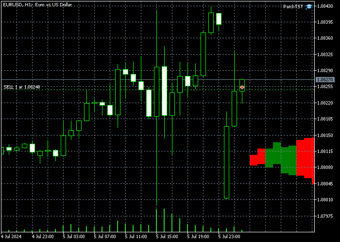
Please note that if you do not see the newly drawn bars to the right, you may need to click the "Shift end of chart from right border" button.

Conclusion

In this article, we took a step-by-step approach to training the PatchTST model, which was introduced in 2023. We got a general sense of how the PatchTST algorithm works. The base code had some issues, related to ONNX conversion. Specifically, the "Unfold" operator is not supported, so we resolved this issue to make the code more ONNX-friendly. We also kept the purpose of the article trader-friendly by focusing on the basics of the model, pulling the data, training the model, and getting a prediction for the next 24 hours. Then we implemented the prediction in MQL5, so we can use the fully trained model with our favorite indicators and expert advisors. I am delighted to share all my code with the MQL community in the attached zip file. Please let me know if you have any questions or comments.