
Auto detection of extreme points based on a specified price variation
Introduction
Many popular trading strategies are based on the use of different graphical patterns: head and shoulders, double top/double bottom and others. Some strategies also analyze the divergence of extreme points on the charts. When automating such trading systems, the necessity arises to find, process and interpret peaks and bottoms on charts. Existing tools do not always allow us to find extreme points according to the established criteria. The article presents efficient algorithms and program solutions for finding and processing extreme points on price charts depending on a price variation.
1. Existing tools for searching for extreme points
1.1. Fractals and similar toolsFractals are popular tools for finding extreme points. They allow finding the price Highs and Lows for the series of 5 bars (Fig. 1). Extreme points are defined both during strong and weak price movements. If a timeframe is selected correctly, the fractals may show good results, though they are strongly affected by market conditions.
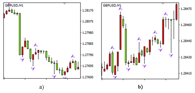
Fig. 1. Results of using fractals: extreme points with a relative size from 140 to 420 pips when a trend is present (a), extreme points during a flat movement, the relative size is no more than 50 pips (b)
In the second case, the relative size of the extreme points (price change from one extreme point to another) may not exceed a few pips. Such insignificant peaks and bottoms are usually not considered when trading manually. Switching between timeframes does not allow sorting out insignificant extreme points — they are still defined during a long flat.
There may also be an issue of an opposite kind: not all extreme points may be defined. If there are some considerable market volatility with a great number of peaks and bottoms within a short time interval, they will not be detected. The fractals are able to detect only 2 extreme points within a time interval defined by 5 bars of the current timeframe. Thus, we cannot recommend the fractals for auto detection of all or the majority of critical extreme points during an automated trading.
The tools described in the article "Thomas DeMark's contribution to technical analysis" have the same drawbacks as the fractals. If we select a large range for searching for extreme points, many of them may be ignored. If the range is too small, some insignificant extreme points may also be defined. In any case, while processing the results, we either have to manually optimize the parameters all the time discarding insignificant Highs and Lows, or develop a special algorithm for that.
1.2. Using moving averages when searching for extreme points
Using an average line, like a moving average, as a basis for automating the search for extreme points seems potentially viable. The search is performed on a specified number of bars if the price deviates from the average line for a distance predefined in points. The tool allows sorting out insignificant peaks and bottoms looking better than the fractals. However, it still does not solve the issue of detecting closely-spaced Highs and Lows (Fig. 2, a).
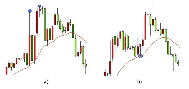
Fig. 2. Using moving averages when searching for extreme points: the two extreme points are defined as one (a), the extreme point located in close proximity to the moving average is ignored (b)
We may use moving averages and fractals together. The moving average is used to sort out insignificant extreme points, while fractals are used to conduct a search within a specified interval. However, this approach does not eliminate all issues as well. We still need to constantly select optimal range parameters. Otherwise, only one extreme point will be defined out of the two closely-spaced ones (Fig. 2, a).
There is also another issue related to this particular method. During the high volatility, a moving average may ignore such a signal depending on a timeframe. In this case (Fig. 2, b), the bottom between the two peaks and near the moving average is not detected. Such occasions are quite rare on the market but they do raise questions about the correct selection of the moving average range.
Thus, the methods of searching for extreme points as well as their modifications described above have drawbacks and require additional programming solutions. Let's consider the issues arising when searching for extreme points as well as the algorithms allowing to solve them in more details.
2. Issues and ambiguities arising when searching for extreme points
2.1. Selecting the variation range for searching for peaks and bottomsExisting strategies and tactics may use extreme points implicitly or explicitly. Finding extreme points is often an arbitrary task: different persons may detect and highlight different peaks and bottoms on the same chart. Let's examine one of well-known graphical patterns – the double top.

Fig. 3. The double top pattern
The two charts (Fig. 3) contain the same pattern. However, we may either detect it or not depending on the extreme points variation range. On the first chart, the first peak is followed by the bottom which in turn is followed by the second peak. Accordingly, if there had been no bottom between the peaks, we would not have been able to detect the double top pattern. The pattern would have been defined as an ordinary extreme point. The same thing occurs when a bottom is not clearly visible obscuring the double top pattern and complicating its detection. Thus, it is easier to detect the pattern on the first chart as compared to the second, while the only difference between them is the variation between the adjacent extreme points.
Let's consider another example: some strategies define trend as upward if subsequent extreme points (both peaks and bottoms) are located above the previous ones. A downward trend is defined similarly. On Fig. 4, we can define a trend direction using extreme points.
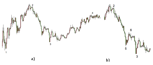
Fig. 4. Oppositely directed price movement on the same chart: uptrend (a), downtrend (b)
The single chart contains both an uptrend and downtrend. In the first case (Fig. 4, a), the extreme points 1, 2, 3 and 4 clearly show a bullish trend. However, if we use the extreme points 2, 5, 6 and 3 (Fig. 4, b), we will see a bearish trend. Thus, it is possible to obtain one of the possible results using different extreme points. Considering this, we may conclude that the variation range has the greatest impact on the extreme points location.
2.2. Efficient separation of adjacent peaks or bottomsThere is also another issue arising when defining extreme points. In order to efficiently define and separate two or more peaks, there should be a bottom between them. This is true both for the first example (finding the top bottom) and for the second one, though the case is even more interesting here. According to the described strategy, we can detect a trend on the charts below (Fig. 5, 6) only after finding extreme points.

Fig. 5. Detecting peaks and bottoms during long-term investments

Fig. 6. Detecting insignificant peaks and bottoms
If there are no bottoms separating peaks (and vice versa), the strategy cannot work according to the specified criteria, though an uptrend can be seen on the chart. Let's consider a typical example. During a bullish trend, each peak is higher than the previous one. If there is no bottom between them or if it is not clearly seen, only the highest peak is defined as an extreme point. If extreme points are defined relative to an average line (like a moving average), the task of separating two adjacent peaks or bottoms remains relevant. In order to separate two peaks, we should use an extreme point between them.
Thus, we may apply the following assumption to all strategies using extreme points implicitly or explicitly: the price moves from a peak to a bottom and from a bottom to a peak both when moving forward (to the future) and backward. If we do not use this assumption, then, depending on the subjective point of view, the two peaks on the price chart:
- are either detected,
- or only the highest peak is detected,
- or neither of them is detected.
The same is true for bottoms. This assumption allows us to develop the algorithm for the accurate search for extreme points using a selected variation range.
2.3. Defining the first extreme pointThe third issue is also related to a price variation and occurs when defining the first extreme point. For any trading tactics or strategy, the most recent extreme points are more important than the older ones. As we have already found out, defining a single extreme point affects the location of adjacent peaks and bottoms. Therefore, if we select an extreme point at some distance from the current time, the obtained results are more strongly affected by more distance historical data and to a much lesser degree affected by the most recent price fluctuations. This issue is present when using ZigZag. Location of the recent extreme points does not depend much on the last price fluctuations.
However, the situation is completely different when searching for extreme points from the end of the chart. In this case, we should first find a peak or a bottom that is the nearest to the chart's end, and all the others are defined unambiguously. Depending on an applied strategy and a selected variation range, three options can be used:
- find the nearest peak,
- find the nearest bottom,
- find the nearest extreme point (either a peak, or a bottom).
Let's consider finding the nearest extreme point. After selecting a certain variation range, we are able to accurately define the first nearest extreme point. However, this occurs with a certain delay that may have a negative impact on the strategy operation. In order to "see" an extreme point, we need to define the price change specified by a variation range relative to that point. Price change takes some time, hence the delay. We can also use the last known price value as an extreme point, although it is unlikely that it will actually turn out to be a peak or a bottom.
In this case, it seems reasonable to find the first extreme point using an additional ratio as a fractional part of the variation range used for finding other extreme points. For example, let's select the value of 0.5.
The selected additional ratio value defines a minimum price change from the current value to the minimum price for the nearest bottom (the maximum price for the nearest peak) allowing us to define this bottom (peak) as an extreme point. If the variation between the current and extreme values for the nearest peak (bottom) is less than the specified value, such an extreme point is not defined. In this case, the detected first extreme point will probably turn out to be a peak or a bottom. At the same time, we also solve the issue of the early detection of extreme points, as well as their subsequent analysis and (if necessary) opening deals.
Let's consider an example with a variation range set to 140 pips. An additional ratio is to be used for detecting the first extreme point. In the first case, it is equal to 0.9 (Fig. 7, a), in the second, it is 0.7 (Fig. 7, b). Here, the value of the additional ratio defines the minimum price variation in pips allowing us to detect the first extreme point. In the first case, the variation is 126 pips, while for the second case, it is 98 pips. The same chart is considered in both cases. The vertical line indicates the current time period, for which calculation is performed. Extreme points detected within this period are shown as dots.
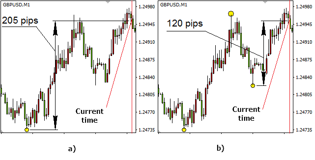
Fig. 7. The influence of the additional ratio on defining the extreme points: for the value of 0.9 (126 pips), the first extreme point is detected at the variation of 205 pips (a), for the value of 0.7 (98 pips), the first extreme point is detected at the variation of 120 pips, while the remaining two ones are detected according to the specified variation range (b)
The selected additional ratio value for the first case helped define the first bottom only at the range of 205 pips, while the minimum price variation is 126 pips. For the second case, in case of the additional ratio equal to 0.7 (98 pips), the first bottom is defined at the variation of 120 pips relative to the current price. The two subsequent extreme values are detected according to the specified variation range equal to 140 pips. Accordingly, the price variation between the first bottom and subsequent peak slightly exceeds 140 pips. The second bottom is also defined by the price variation exceeding 140 pips though relative to the detected peak.
As we can see, the additional ratio significantly affects the location of the first detected extreme point. It may also affect its type as well. For various values (from 0 to 1), either a peak or a bottom may be detected first on the same chart. The first two extreme points detected for the second case (Fig. 7 b), were not defined in the first one.
In case of an even lower ratio, the first extreme point is defined faster. In the second case (Fig. 7 b), with the additional ratio of 0.4, the first detected extreme value can be defined 5 bars earlier (5 minutes earlier on the current timeframe scale).
3. The algorithmic solutions for extreme points searching tasks and their implementation
Let's start from the selection of the price range for building extreme points. Obviously, the bar sizes and extreme point parameters vary greatly depending on a timeframe. The presence and absence of peaks/bottoms is also affected by a trend, time of day and other factors. Existing indicators, like fractals and similar tools, allow us to find extreme points on any timeframe regardless of whether a trend is present. If we use a moving average when searching for peaks and bottoms, the size of extreme points relative to the moving average may comprise 2 points as well as 100. Should we pay attention to 2 point extreme values in intraday trading? Probably, no. In case of a long-term investment, we are not interested in extreme values less than 20 points either, regardless of a timeframe.
This is why we need the "variation range" term meaning a minimum value. A moving average can be used as a reference point allowing us to define the distance to an extreme point and limit its minimum value. However, the moving average period significantly affects the position of the detected peaks and bottoms making it difficult to select a certain period as a reference.
Therefore, let's assume from now on that the price moves from peak to bottom and back, and the variation range is defined as a minimum price change in points between the two neighboring extreme points — the peak and the bottom. If some of the extreme points is defined already, the neighboring one should be located at a distance no less than the one specified by the variation range. This allows us to define extreme points regardless of a timeframe and a trend. The tool is perfectly suitable both for intraday trading and long-term investment.
Let's consider its operation algorithm. First, let's visually define the extreme points using the same chart, though in the first chart, the variation range is 60 pips (Fig. 8), while in the second chart it is 30 pips (Fig. 9). Let's also assume that the first extreme point is already detected (point 1) and we are searching for the preceding ones.
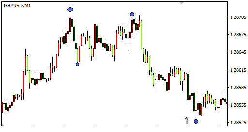
Fig. 8. Using the variation range of 60 pips
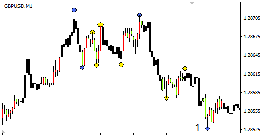
Fig. 9. Using the variation range of 30 pips
The search for extreme points is performed from the end of the chart (from the point 1). In the first case, 4 extreme points were found in the displayed range, in the second case, there were 10 extreme points detected on the same interval. When increasing the variation range on a specified part of the chart, extreme points are not detected at all. Therefore, we should be realistic when selecting the extreme point search range and take the market volatility and timeframe into account. Here, the range is a number of bars, on which the search is performed.
Keeping in mind all that we mentioned above, let's introduce the iteration algorithm for searching for extreme points. Why iteration? The first peak should always be followed by the bottom, the second peak goes after it, etc. If the second peak is not found (the chart does not move upwards), the bottom's position is redefined, and it is moved farther and farther away on the time series. The first peak's position (as well as any other extreme point's one) can be corrected the same way. We should also discard the cases when the same bar is defined both as a peak and as a bottom.
Of course, this approach requires a large amount of calculation. I advise applying it when searching for several extreme points. The smaller the number of points, the faster the program works. The calculation speed is also affected by a search range. This search is justified, since it allows you to define certain peaks and bottoms at the maximum impact of the most recent price fluctuations. If you need to find multiple extreme points, I recommend using ZigZag.
3.2 Indicator implementationThe iteration algorithm code presented below uses a small number of iterations for better performance. This simplification does not cause significant loss of extreme point detection quality. The main incoming parameters — the range for searching extreme points and the variation range.
input double delta_points=160; // variation range defining the minimum distance between a peak and a bottom in points
input double first_extrem=0.9; // additional ratio for searching for the first extreme value
input double reload_time=5; // time interval, after which the indicator values are recalculated, in seconds
The program body contains three nested loops necessary for defining four extreme points. Only the first bottom and related extreme points are defined in this part of the program. Defining the first peak and related extreme points is implemented in a similar way.
datetime Time[];
ArraySetAsSeries(Low,true);
int copied1=CopyLow(Symbol(),0,0,bars+2,Low);
ArraySetAsSeries(High,true);
int copied2=CopyHigh(Symbol(),0,0,bars+2,High);
ArraySetAsSeries(Time,true);
int copied3=CopyTime(Symbol(),0,0,bars+2,Time);
double delta=delta_points*Point(); // variation range between extreme points in absolute terms
int j,k,l;
int j2,k2,l2;
double j1,k1,l1;
int min[6]; // array defining bottoms, the value corresponds to the bar index for a detected extreme point
int max[6]; // array defining the peaks, the value corresponds to the bar index for a detected extreme point
int mag1=bars;
int mag2=bars;
int mag3=bars;
int mag4=bars;
j1=SymbolInfoDouble(Symbol(),SYMBOL_BID)+(1-first_extrem)*delta_points*Point();
// when searching for the first extreme point, the additional ratio defines the minimum price, below which the first bottom is to be located
j2=0; // at the first iteration, the search is performed beginning from the last history bar
for(j=0;j<=15;j++) // loop defining the first bottom - min[1]
{
min[1]=minimum(j2,bars,j1);
//define the nearest bottom within the specified interval
j2=min[1]+1; // at the next iteration, the search is performed from the already detected bottom min[1]
j1=Low[min[1]]+delta;
//Low price for the bottom detected on the subsequent iteration should be lower than the Low price for the bottom found at the current iteration
k1=Low[min[1]];
//Low price for the bottom when searching for the next extreme point defines the High price, above which the peak should be located
k2=min[1]; //search for the peak located after the bottom is performed from the detected bottom min[1]
for(k=0;k<=12;k++) // loop defining the first peak - max[1]
{
max[1]=maximum(k2,bars,k1);
//--- define the nearest peak in a specified interval
k1=High[max[1]]-delta;
//High price for the next iteration should exceed the High price for the peak detected on the current iteration
k2=max[1]+1; // at the next iteration, the search is performed from the already detected peak max[1]
l1=High[max[1]];
//High price for the extreme point when searching for the next bottom defines the Low price, below which the bottom should be located
l2=max[1]; // search for the bottom located after the peak is performed from the detected peak max[1]
for(l=0;l<=10;l++) // loop defining the second bottom - min[2] and the second peak max[2]
{
min[2]=minimum(l2,bars,l1);
//---define the nearest bottom within the specified interval
l1=Low[min[2]]+delta;
//Low price for the bottom detected on the subsequent iteration should be lower than the Low price for the bottom found at the current iteration
l2=min[2]+1; // at the next iteration, the search is performed from the already detected bottom min[2]
max[2]=maximum(min[2],bars,Low[min[2]]);
//define the nearest peak in a specified interval
if(max[1]>min[1] && min[1]>0 && min[2]>max[1] && min[2]<max[2] && max[2]<mag4)
//sort out coinciding extreme values and special cases
{
mag1=min[1]; // at each iteration, locations of the detected extreme values are saved if the condition is met
mag2=max[1];
mag3=min[2];
mag4=max[2];
}
}
}
}
min[1]=mag1; // extreme points are defined, otherwise the 'bars' value is assigned to all variables
max[1]=mag2;
min[2]=mag3;
max[2]=mag4;
Finding the nearest bar, the Low price of which is below the specified value (or the High price of which exceeds the specified value) is a quite simple task and is made into a separate function.
//the function defines the nearest bottom on the specified interval. The bottom is located below price0 at a distance more than the variation range
{
double High[],Low[];
ArraySetAsSeries(Low,true);
int copied4=CopyLow(Symbol(),0,0,bars+2,Low);
int i,e;
e=bars;
double pr=price0-delta_points*Point(); // the price, below which the bottom with the added variation range should be located
for(i=a;i<=b;i++) // search for the bottom within the range specified by a and b parameters
{
if(Low[i]<pr && Low[i]<Low[i+1]) // define the nearest bottom, after which the price growth starts
{
e=i;
break;
}
}
return(e);
}
int maximum(int a,int b,double price1)
//--- the function defines the nearest peak on the specified interval. The bottom is located above price1 at a distance more than the variation range
{
double High[],Low[];
ArraySetAsSeries(High,true);
int copied5=CopyHigh(Symbol(),0,0,bars+2,High);
int i,e;
e=bars;
double pr1=price1+delta_points*Point(); // the price, above which the peak with the added variation range should be located
for(i=a;i<=b;i++) // search for the peak within the range specified by a and b parameters
{
if(High[i]>pr1 && High[i]>High[i+1]) // define the nearest peak, after which the price starts falling
{
e=i;
break;
}
}
return(e);
}
The task of finding extreme points is solved but only at a first approximation. We should consider that the peak (located between the two bottoms) found using the algorithm may not be the highest one within the specified algorithm. Since the search started from the end of the chart, the position of peaks and bottoms should be clarified from the end for the first, second, third and subsequent extreme points. Verification and correction of the peak and bottom positions are made as separate functions. The implementation of the extreme points position clarification looks as follows:
min[1]=check_min(min[1],max[1]); // verify and correct the position of the first bottom within the specified interval
max[1]=check_max(max[1],min[2]); // verify and correct the position of the first peak within the specified interval
min[2]=check_min(min[2],max[2]); // verify and correct the position of the second bottom within the specified interval
int check_min(int a,int b)
// the function for verifying and correcting the bottom position within the specified interval
{
double High[],Low[];
ArraySetAsSeries(Low,true);
int copied6=CopyLow(Symbol(),0,0,bars+1,Low);
int i,c;
c=a;
for(i=a+1;i<b;i++) // when searching for the bottom, all bars specified by the range are verified
{
if(Low[i]<Low[a] && Low[i]<Low[c]) // if the bottom located lower is found
c=i; // the bottom location is redefined
}
return(c);
}
//--- the function for verifying and correcting the peak position within the specified interval
{
double High[],Low[];
ArraySetAsSeries(High,true);
int copied7=CopyHigh(Symbol(),0,0,bars+1,High);
int i,d;
d=a;
for(i=(a+1);i<b;i++) // when searching for the bottom, all bars specified by the range are verified
{
if(High[i]>High[a] && High[i]>High[d]) // if the peak located higher is found
d=i; // the peak location is redefined
}
return(d);
}
If four extreme points are found, we need to clarify the positions of only the first three ones. The verification and correction function works within the range defined for the current extreme point using its own position and the position of the following extreme point. After the clarification, we can be sure that found extreme points correspond to the set criteria.
After that, the search for the first peak is performed from the chart's end and the positions of the first peak and bottom are compared. As a result of performed calculations, we obtain the positions of the first extreme point and related extreme points that are closest to the chart's end.
Let's dwell once again on finding the first extreme point. I have already offered to introduce the additional search ratio — fractional part from the variation range, for example 0.7. At the same time, its high values (0.8…0.9) allow us to accurately define the first extreme point with a slight delay, while its low values (0.1…0.25) decrease the delay to the minimum but the accuracy is seriously diminished in that case. Accordingly, the additional ratio value should be selected depending on the applied strategy.
Detected peaks and bottoms are shown as arrows. The arrows display the extreme points coordinates (time series and High/Low price for a detected peak/bottom). Since this requires a lot of calculations, the program features the input parameter setting the interval used to re-calculate the indicator values. If no peaks and bottoms are found, the indicator generates an appropriate message. The implementation of the graphical display of extreme points looks as follows:
if(min[1]<Max[1]) // if the bottom is located closer, its position as well as the positions of the related extreme values are displayed
{
ObjectDelete(0,"id_1"); // delete the labels made during the previous stage
ObjectDelete(0,"id_2");
ObjectDelete(0,"id_3");
ObjectDelete(0,"id_4");
ObjectDelete(0,"id_5");
ObjectDelete(0,"id_6");
ObjectCreate(0,"id_1",OBJ_ARROW_UP,0,Time[min[1]],Low[min[1]]); // highlight the first bottom
ObjectSetInteger(0,"id_1",OBJPROP_ANCHOR,ANCHOR_TOP);
//--- for the first detected bottom, the binding is performed by its position on the time series and the Low price
ObjectCreate(0,"id_2",OBJ_ARROW_DOWN,0,Time[max[1]],High[max[1]]); // highlight the first peak
ObjectSetInteger(0,"id_2",OBJPROP_ANCHOR,ANCHOR_BOTTOM);
//--- for the detected peak, the binding is performed by its position on the time series and the High price
ObjectCreate(0,"id_3",OBJ_ARROW_UP,0,Time[min[2]],Low[min[2]]); // highlight the second bottom
ObjectSetInteger(0,"id_3",OBJPROP_ANCHOR,ANCHOR_TOP);
//--- for the second detected bottom, the binding is performed by its position on the time series and the Low price
}
if(min[1]>Max[1]) // if the peak is located closer, its position as well as the positions of the related extreme values are displayed
{
ObjectDelete(0,"id_1"); // delete the labels made during the previous stage
ObjectDelete(0,"id_2");
ObjectDelete(0,"id_3");
ObjectDelete(0,"id_4");
ObjectDelete(0,"id_5");
ObjectDelete(0,"id_6");
ObjectCreate(0,"id_4",OBJ_ARROW_DOWN,0,Time[Max[1]],High[Max[1]]); // define the first peak
ObjectSetInteger(0,"id_4",OBJPROP_ANCHOR,ANCHOR_BOTTOM);
//for the first detected peak, the binding is performed by its position on the time series and the High price
ObjectCreate(0,"id_5",OBJ_ARROW_UP,0,Time[Min[1]],Low[Min[1]]); // highlight the first bottom
ObjectSetInteger(0,"id_5",OBJPROP_ANCHOR,ANCHOR_TOP);
//for the detected bottom, the binding is performed by its position on the time series and the Low price
ObjectCreate(0,"id_6",OBJ_ARROW_DOWN,0,Time[Max[2]],High[Max[2]]); // define the second peak
ObjectSetInteger(0,"id_6",OBJPROP_ANCHOR,ANCHOR_BOTTOM);
//for the second detected peak, the binding is performed by its position on the time series and the High price
}
if(min[1]==Max[1]) Alert("Within the specified range, ",bars," no bars and extreme points found");
// if no extreme points found, the appropriate message appears
When de-initializing the indicator, the objects defining peaks and bottoms are removed.
The provided algorithms have been used to develop the custom indicator that searches for extreme points and highlights them on the chart (Fig. 10).
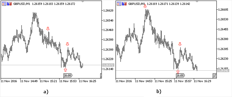
Fig. 10. The indicator operation results: the variation range 120 pips (a), the variation range 160 pips (b)
The obtained results are defined by the variation range. For the value of 120 pips and less (Fig. 10, a), the extreme points are located quite close to each other and the range size is of no great importance. For the value of 160 pips and more (Fig. 10, b), the extreme points are located far enough. This should be noted, when selecting the search range. In case of a flat market, the optimally selected range allows us to automatically find peaks and bottoms in case of a weak movement and sort out (skip) extreme points separated by very large time intervals.
3.3 The Expert Advisor implementing the divergence strategy between MACD histogram and pricesThe provided algorithms can be implemented for a variety of strategies. The scale_factor indicator operation results are well-suited for working with graphical models, like head and shoulders, double top, double bottom, etc. They can be used in the strategies applying peaks and bottoms divergences for price charts and indicators. One of the examples is an Expert Advisor (EA) that follows the price chart and MACD histogram divergence strategy. This strategy is described in literature in details (see "Trading for a Living" by Alexander Elder).
According to the strategy, if the price goes upwards and forms a new peak above the previous one but the MACD peak is lower than the previous one, we have a sell signal.
If the price moves downwards forming a new bottom below the previous one but the MACD bottom is higher than the previous one, we have a buy signal.
The EA implementing this algorithm accurately detects the necessary peaks and bottoms according to the variation range primarily focusing on the latest changes on the price chart.
The incoming parameters — the range for searching extreme points and the variation range. It is also necessary to set the minimum price divergence for the last two peaks during the upward price movement (for the last two bottoms during the downward price movement), minimum deviation of MACD histogram for extreme points. The risk and the additional ratio are set per each trade in the deposit currency. The guard_points parameter defines the additional stop loss shift relative to the minimum price value for the nearest bottom if a long position is opened. Accordingly, a stop loss is shifted upwards when opening a short position. It is also possible to deduce the parameters of the detected extreme points when opening trades (show_info=1).
input double delta_points=160; // variation range defining the minimum distance between a peak and a bottom in points
input double first_extrem=0.9; // additional ratio for searching for the first extreme value
input int orderr_size=10; // risk per each trade
input double macd_t=0.00002; // minimum MACD histogram deviation
input double trend=100; // minimum price deviation for the nearest two peaks/bottoms
input double guard_points=30; // shift the stop loss
input int time=0; // time delay in seconds
input int show_info=0; // display data about extreme points
Calculations can be performed per each tick. The same is true for trades. The strategy works well even with a time delay. After defining the main parameters in absolute terms, we should pass to searching for extreme points. The first part of the program allows finding extreme points in case the first of them is a bottom. After that, their status is clarified. The second part of the code allows finding extreme points for the case when a peak is located the first from the chart's end. The peaks and bottoms parameters are clarified at the next step.
{
Sleep(1000*time); // introduce the time delay
double High[],Low[];
ArraySetAsSeries(Low,true);
int copied1=CopyLow(Symbol(),0,0,bars+2,Low);
ArraySetAsSeries(High,true);
int copied2=CopyHigh(Symbol(),0,0,bars+2,High);
ArraySetAsSeries(Time,true);
int copied3=CopyTime(Symbol(),0,0,bars+2,Time);
MqlTick last_tick;
double Bid=last_tick.bid;
double Ask=last_tick.ask;
double delta=delta_points*Point(); // variation value in absolute terms
double trendd=trend*Point(); // minimum price deviation for the nearest two peaks/bottoms in absolute terms
double guard=guard_points*Point(); // stop loss shift in absolute terms
int j,k,l;
int j2,k2,l2;
double j1,k1,l1;
int min[6]; // array defining bottoms if the first detected extreme value is a bottom, the value corresponds to the bar index for a detected extreme point
int max[6]; // array defining peaks if the first detected extreme value is a bottom, the value corresponds to the bar index for a detected extreme point
int Min[6]; // array defining bottoms if the first detected extreme value is a peak, the value corresponds to the bar index for a detected extreme
int Max[6]; // array defining peaks if the first detected extreme value is a peak, the value corresponds to the bar index for a detected extreme point
int mag1=bars;
int mag2=bars;
int mag3=bars;
int mag4=bars;
j1=SymbolInfoDouble(Symbol(),SYMBOL_BID)+(1-first_extrem)*delta_points*Point();
// when searching for the first extreme point, the additional ratio defines the minimum price, below which the first bottom is to be located
j2=0; // at the first iteration, the search is performed beginning from the last history bar
for(j=0;j<=15;j++) // loop defining the first bottom - min[1]
{
min[1]=minimum(j2,bars,j1);
//define the nearest bottom within the specified interval
j2=min[1]+1; //at the next iteration, the search is performed from the already detected bottom min[1]
j1=Low[min[1]]+delta;
//--- Low price for the bottom detected on the subsequent iteration should be lower than the Low price for the bottom found at the current iteration
k1=Low[min[1]];
//Low price for the bottom when searching for the next extreme point defines the High price, above which the peak should be located
k2=min[1]; // search for the peak located after the bottom is performed from the detected bottom min[1]
for(k=0;k<=12;k++) // loop defining the first peak - max[1]
{
max[1]=maximum(k2,bars,k1);
//--- define the nearest peak in a specified interval
k1=High[max[1]]-delta;
//--- High price for the next iteration should exceed the High price for the peak detected on the current iteration
k2=max[1]+1; // at the next iteration, the search is performed from the already detected peak max[1]
l1=High[max[1]];
//--- High price for the extreme point when searching for the next bottom defines the Low price, below which the bottom should be located
l2=max[1]; // search for the bottom located after the peak is performed from the detected peak max[1]
for(l=0;l<=10;l++) // loop defining the second bottom - min[2] and the second peak max[2]
{
min[2]=minimum(l2,bars,l1);
//--- define the nearest bottom within the specified interval
l1=Low[min[2]]+delta;
//Low price for the bottom detected on the subsequent iteration should be lower than the Low price for the bottom found at the current iteration
l2=min[2]+1; //at the next iteration, the search is performed from the already detected bottom min[2]
max[2]=maximum(min[2],bars,Low[min[2]]);
//define the nearest peak in a specified interval
if(max[1]>min[1] && min[1]>0 && min[2]>max[1] && min[2]<max[2] && max[2]<mag4)
//--- sort out coinciding extreme values and special cases
{
mag1=min[1]; // at each iteration, locations of the detected extreme values are saved if the condition is met
mag2=max[1];
mag3=min[2];
mag4=max[2];
}
}
}
}
//--- extreme points are defined, otherwise the 'bars' value is assigned to all variables
min[1]=mag1;
max[1]=mag2;
min[2]=mag3;
max[2]=mag4;
//--- verify and correct the extreme points position within the specified interval
max[1]=check_max(max[1],min[2]);
min[2]=check_min(min[2],max[2]);
//---------------------------------------------------------------------------------------------------------------
mag1=bars;
mag2=bars;
mag3=bars;
mag4=bars;
j1=SymbolInfoDouble(Symbol(),SYMBOL_BID)-(1-first_extrem)*delta_points*Point();
// when searching for the first extreme point, the additional ratio defines the maximum price, above which the first peak is to be located
j2=0; // at the first iteration, the search is performed beginning from the last history bar
for(j=0;j<=15;j++) // loop defining the first peak - Max[1]
{
Max[1]=maximum(j2,bars,j1);
//define the nearest peak within the specified interval
j1=High[Max[1]]-delta;
//High price for the next iteration should exceed the High price for the peak detected on the current iteration
j2=Max[1]+1; // at the next iteration, the search is performed from the already detected peak Max[1]
k1=High[Max[1]];
//High price for the extreme point when searching for the next bottom defines the Low price, below which the bottom should be located
k2=Max[1]; // search for the bottom located after the peak is performed from the detected peak max[1]
for(k=0;k<=12;k++) //loop defining the first peak - Min[1]
{
Min[1]=minimum(k2,bars,k1);
//--- define the nearest bottom within the specified interval
k1=Low[Min[1]]+delta;
//Low price for the bottom detected on the subsequent iteration should be lower than the Low price for the bottom found at the current iteration
k2=Min[1]+1; // at the next iteration, the search is performed from the already detected bottom min[1]
l1=Low[Min[1]];
//---Low price for the bottom when searching for the next extreme point defines the High price, above which the peak should be located
l2=Min[1]; // search for the peak located after the bottom is performed from the detected bottom min[1]
for(l=0;l<=10;l++)//loop defining the second peak - Max[2] and the second bottom Min[2]
{
Max[2]=maximum(l2,bars,l1);
//define the nearest peak within the specified interval
l1=High[Max[2]]-delta;
//High price for the next iteration should exceed the High price for the peak detected on the current iteration
l2=Max[2]+1; //at the next iteration, the search is performed from the already detected peak Max[2]
Min[2]=minimum(Max[2],bars,High[Max[2]]);
//---define the nearest bottom within the specified interval
if(Max[2]>Min[1] && Min[1]>Max[1] && Max[1]>0 && Max[2]<Min[2] && Min[2]<bars)
//--- sort out coinciding extreme values and special cases
{
mag1=Max[1]; // at each iteration, locations of the detected extreme values are saved if the condition is met
mag2=Min[1];
mag3=Max[2];
mag4=Min[2];
}
}
}
}
Max[1]=mag1; // extreme points are defined, otherwise the 'bars' value is assigned to all variables
Min[1]=mag2;
Max[2]=mag3;
Min[2]=mag4;
Max[1]=check_max(Max[1],Min[1]); // verify and correct the positions of the extreme points within the specified interval
Min[1]=check_min(Min[1],Max[2]);
Max[2]=check_max(Max[2],Min[2]);
Further on, we may use either the first passed peak or the first detected bottom, however, it seems more reasonable to use the nearest extreme point, as well as peaks and bottoms obtained based on it.
For both cases, the lot size as well as the indicator values corresponding to the extreme point positions are calculated. The condition for correct extreme points detection and the absence of open positions is verified.
If there is a divergence between the extreme points prices and the MACD histogram and it is not less than the values set by the inputs, the appropriate position is opened. The divergences should be oppositely directed.
//calculate the lot when buying
double lot_sell=NormalizeDouble(0.1*orderr_size/(NormalizeDouble(((High[Max[1]]-SymbolInfoDouble(Symbol(),SYMBOL_ASK)+guard)*10000),0)+0.00001),2);
//--- calculate the lot when selling
int index_handle=iMACD(NULL,PERIOD_CURRENT,12,26,9,PRICE_MEDIAN);
double MACD_all[];
ArraySetAsSeries(MACD_all,true);
int copied4=CopyBuffer(index_handle,0,0,bars+2,MACD_all);
double index_min1=MACD_all[min[1]];
double index_min2=MACD_all[min[2]];
//---calculate the indicator values corresponding to the extreme points if the first extreme point is a bottom
double index_Max1=MACD_all[Max[1]];
double index_Max2=MACD_all[Max[2]];
//calculate the indicator values corresponding to the extreme points if the first extreme point is a peak
bool flag_1=(min[2]<bars && min[2]!=0 && max[1]<bars && max[1]!=0 && max[2]<bars && max[2]!=0); //Check the condition of the correct extreme point condition
bool flag_2=(Min[1]<bars && Min[1]!=0 && Max[2]<bars && Max[2]!=0 && Min[2]<bars && Min[2]!=0);
bool trend_down=(Low[min[1]]<(Low[min[2]]-trendd));
bool trend_up=(High[Max[1]]>(High[Max[2]]+trendd));
//---difference between extreme points price values should not be less than a set value
openedorder=PositionSelect(Symbol()); //verify the condition for the absence of open positions
if(min[1]<Max[1] && trend_down && flag_1 && !openedorder && (index_min1>(index_min2+macd_t)))
//if the first extreme point is a bottom, a buy trade is opened
//difference between MACD values for extreme points is not less than the value of macd_t set as an input
// trade is opened in case of an oppositely directed movements of the price and the indicator calculated based on extreme points
{
if(show_info==1) Alert("For the last",bars," bars, the distance in bars to the nearest bottom and extreme points",min[1]," ",max[1]," ",min[2]);
//--- display data on extreme points
MqlTradeResult result={0};
MqlTradeRequest request={0};
request.action=TRADE_ACTION_DEAL;
request.magic=123456;
request.symbol=_Symbol;
request.volume=lot_buy;
request.price=SymbolInfoDouble(Symbol(),SYMBOL_ASK);
request.sl=Low[min[1]]-guard;
request.tp=MathAbs(2*SymbolInfoDouble(Symbol(),SYMBOL_BID)-Low[min[1]])+guard;
request.type=ORDER_TYPE_BUY;
request.deviation=50;
request.type_filling=ORDER_FILLING_FOK;
OrderSend(request,result);
}
if(min[1]>Max[1] && trend_up && flag_2 && !openedorder && (index_Max1<(index_Max2-macd_t)))
//if the first extreme point is a peak, a sell trade is opened
//difference between MACD values for extreme points is not less than the value of macd_t set as an input
// trade is opened in case of an oppositely directed movements of the price and the indicator calculated based on extreme points
{
if(show_info==1) Alert("For the last ",bars," bars, the distance in bars to the nearest peak and extreme points",Max[1]," ",Min[1]," ",Max[2]);
//---display data on extreme points
MqlTradeResult result={0};
MqlTradeRequest request={0};
request.action=TRADE_ACTION_DEAL;
request.magic=123456;
request.symbol=_Symbol;
request.volume=lot_sell;
request.price=SymbolInfoDouble(Symbol(),SYMBOL_BID);
request.sl=High[Max[1]]+guard;
request.tp=MathAbs(High[Max[1]]-2*(High[Max[1]]-SymbolInfoDouble(Symbol(),SYMBOL_ASK)))-guard;
request.type=ORDER_TYPE_SELL;
request.deviation=50;
request.type_filling=ORDER_FILLING_FOK;
OrderSend(request,result);
}
When opening a short position, a stop loss is set by the position of the nearest peak, while when opening a long position, it is set by the position of the nearest bottom allowing us to establish realistic targets both during strong price fluctuations and quiet market. In both cases, a take profit is set symmetrical to a stop loss relative to the current price value. In intraday trading, a small variation range is selected, while in long-term investment, it is advisable to set the variation range a few times bigger.
Let's consider the following example of the EA operation (Fig. 11). The main applied parameters: variation range — 160 pips, minimum MACD histogram divergence – 0,0004; minimum price divergence for the two nearest peaks/bottoms – 120 pips and additional ratio – 0.9.
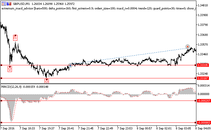
Fig. 11. The EA operation results
First, the EA searches for the last 3 extreme points. At the moment of making a decision to go long, the EA detects one peak and two bottoms (marked as arrows). Unlike the indicator, the EA does not highlight the extreme points. However, we can obtain data on extreme points positions when opening trades by setting show_info to 1.
The price divergence for the 2 nearest bottoms comprises 148 pips exceeding the specified value. The MACD histogram divergence comprises 0.00062 for the same extreme points also exceeding the specified value. Considering the oppositely directed price and indicator movements detected by the last 2 bottoms, the long position is opened in the point defined by the additional ratio (150 pips). If using a lower additional ratio, position could have been opened earlier, thus the profit could have been fixed sooner.
Below are the EA test results (Fig. 12). The maximum impact of macd_t and trend parameters on the profitability has been revealed during the test. The bigger the value of the parameters, the greater the amount of profitable trades in percentage value. However, the increase of profitability happens simultaneously with the decrease of the total number of trades.
For instance, if macd_t = 0.0006 and trend=160 (Fig. 12), 56% of trades have turned out to be profitable out of 44 ones. If macd_t = 0.0004 and trend=120, 84 trades are performed with 51% of them being profitable.
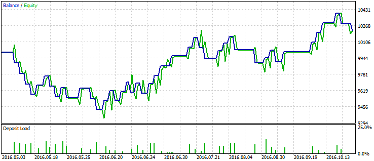
Fig. 12. The EA test results
When optimizing the strategy, the correctly set macd_t and trend parameters are of critical importance. Variation range and additional value also affect the trades parameters. The variation range defines the number of detected extreme points and trades. The additional ratio defines how tightly take profit and stop loss are to be located when opening positions.
This strategy, as well as a number of others, may work as correctly as possible only when using the tools proposed above. Otherwise, there may be situations when a trade with a specified take profit and stop loss at 200 points from the current price value is opened based on the signals received when using extreme points of 5 points or less. The significance of such extreme points is very low in this case. In these and many other situations, the conventional tools either define too many insignificant extreme points or do not detect peaks and bottoms at all. Besides, these tools often have issues defining extreme points at the end of a time series.
Conclusion
The algorithms and solutions described in the article make it possible to accurately define extreme points on the price charts depending on the price variation. Obtained results are applicable both when defining the graphical patterns and when implementing trading strategies that use graphical patterns and indicators. The developed tools feature a number of advantages over the well-known solutions. Only critical extreme points are defined regardless of the market situation (trend or flat). Only extreme points exceeding a predefined value are detected. Other peaks and bottoms are ignored. The search for extreme points is performed from the chart's end allowing us to obtain results mostly depending on the recent price fluctuations. These results are not strongly affected by a selected timeframe and are only defined by a specified price variation.
Translated from Russian by MetaQuotes Ltd.
Original article: https://www.mql5.com/ru/articles/2817
Warning: All rights to these materials are reserved by MetaQuotes Ltd. Copying or reprinting of these materials in whole or in part is prohibited.
This article was written by a user of the site and reflects their personal views. MetaQuotes Ltd is not responsible for the accuracy of the information presented, nor for any consequences resulting from the use of the solutions, strategies or recommendations described.
 Graphical interfaces X: Advanced management of lists and tables. Code optimization (build 7)
 An Example of Developing a Spread Strategy for Moscow Exchange Futures
- Free trading apps
- Over 8,000 signals for copying
- Economic news for exploring financial markets
You agree to website policy and terms of use
New article Automatic detection of extreme points based on specific price changes has been published:
Author: Sergey Strutinskiy
Nice thought!
Have you some code in mt4 ?
New article Automatic detection of extreme points based on a specified price variation has been published:
Author: Sergey Strutinskiy
How can I use this indicator in my EA? I didn't see a Buffer for use in ICustom.