Monte Carlo Simulation and Analysis for MetaTrader 5 Backtest Reports

Introduction

You ran a strategy in MetaTrader 5 and got a beautiful equity curve in the Strategy Tester — but when you trade live or forward-test, performance is worse: deeper drawdowns, rare catastrophic sequences, or simply a different trajectory. The core issue is that a single backtest run shows only one possible ordering of the same trades. It does not expose the distribution of possible equity paths or the likelihood of tail events.

This article shows how to bridge that gap. First, I clarify the difference between Monte Carlo simulation (generating many equity curves by shuffling the actual closed trades) and Monte Carlo analysis (extracting actionable statistics from those curves). Then I provide a practical, repeatable Python pipeline that accepts an MetaTrader 5 Strategy Tester HTML report and a sample size, extracts closed-trade PnL and the initial balance, runs many shuffled simulations, and produces both a saved plot (mean equity plus 5–95% bands) and numeric outputs: bust rate, profit rate, and max observed drawdown. The goal is concrete: give you a tool and clear metrics to quantify tail risk and choose an appropriate risk sizing — not another single “pretty” curve. Remember: models are not perfect, but a Monte Carlo workflow makes hidden risks visible and helps you avoid surprises in live trading.

Monte Carlo Simulation and Analysis? Never heard of it

As much as one can interchange the two terms and understand what they mean in different contexts, it's good to know what each term means in most situations.

A Monte Carlo simulation in the context of trading is the process of generating multiple equity curves by shuffling trading data. In the case of a backtest, this mainly involves obtaining the positions taken by the strategy, and shuffling them around to generate the multiple equity curves.

A Monte Carlo analysis on the other hand, is the extraction of data from the Monte Carlo simulation. From the numerous equity curves generated, one can gauge metrics such as max drawdown, how many of the simulations went broke (bust rate), how many were profitable (profit rate) and many more.

Monte Carlo simulation and analysis enable us to quantify a strategy's performance before deploying it live. However, remember that all models are wrong but some are useful. Monte Carlo results help define expected behavior and outliers, but they are not guaranteed. It is just a useful tool to benchmark our strategy’s performance.

To better understand this concept, let us develop such a system to simulate trades taken by a strategy by using the HTML file generated by MQL5 Strategy Tester.

The Setup

The Monte Carlo simulation and analysis system will be coded in Python and a few dependencies will need to be installed beforehand. I am using Linux for this tutorial but I will try my best to link any differing concepts for Windows and Mac users.

First, create a virtual environment so that the project does not accidentally mess up our operating system as well as dependencies for other projects:

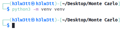
Then activate the virtual environment:

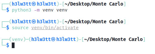
For Windows users, the activation line should be:

venv\Scripts\activate

Once in the virtual environment, a few modules are needed. Start by installing argparse:

pip3 install argparse

Argparse enables one to define what parameters the program requires in the case of a help screen as well as take in inputs directly from the Command Line Interface (CLI) into the program.

Then install matplotlib:

pip3 install matplotlib

Matplotlib is probably the most famous plotting library for Python, and in our case, it will be needed to plot the equity curves.

Next is pandas:

pip3 install pandas

Pandas is used for data manipulation and analysis, and in this program, it will primarily be used to store Profit and Loss numbers (PnL) data in a DataFrame.

Next, lxml:

pip3 install lxml

Lxml is essential for reading data from HTML and XML files. In our case, it will be used to read the PnL data from the HTML report file and provide it to pandas for storage and arrangement.

Last but not least, numpy:

pip3 install numpy

Numpy is used for numerical computations, and in our case, it will be quite useful in the analysis of the multiple equity curves.

With all the modules successfully installed, one can proceed to the code.

The Code

Using your favorite text editor or IDE if you really want to be fancy, make a new file and call it ‘monteCarlo.py’. Honestly, the file name can be whatever you would like it to be but the last part, .py, is necessary for the file to run. Keep that in mind.

Once you’ve done that, open the file and add the following lines of code:

import random                           #For shuffling the PnL
import gc                               #For cleanup
import matplotlib.pyplot as plt         #For plotting the equity curves
import pandas as pd                     #For data extraction and formatting
import numpy as np                      #For calculations on extracted data
import argparse                         #For input from CLI as well as help menu

I had explained most of this earlier, except random and gc. Gc is used for garbage collection, basically reclaiming memory from objects that are no longer in use and by doing so, it makes the program a bit more efficient in terms of memory. I will explain random a bit later when I show its use case.

Next, setting up argparse:

# Argparse stuff
parser = argparse.ArgumentParser(
        prog="MonteCarloSimulator",
        formatter_class=argparse.RawDescriptionHelpFormatter,
        description="""
==================================================
|  MONTE CARLO SIMULATION AND ANALYSIS FOR MQL5  |
==================================================

Extracts PnL from MQL5 HTML Report files and runs a Monte Carlo simulation and analysis.
        """,
        epilog="""
Examples: python3 monteCarlo.py myReport.html 1000 myReport.png
          python3 monteCarlo.py path_to_my_report/myReport.html 100000 path_to_save/myReport.png
        """
)                                                                                               #Setting up the help screen

parser.add_argument("report", help="Path to MQL5 HTML report")                                  #Report argument
parser.add_argument("sampleSize", help="Sample Size/ Number of Runs for analysis", type=int)    #Sample Size argument
parser.add_argument("output", help="Name and path for .png output")                             #Name & location for output file

args = parser.parse_args()                                                                      #Stores data input from CLI

This may be a bit hard to understand but its easier to see it in action:

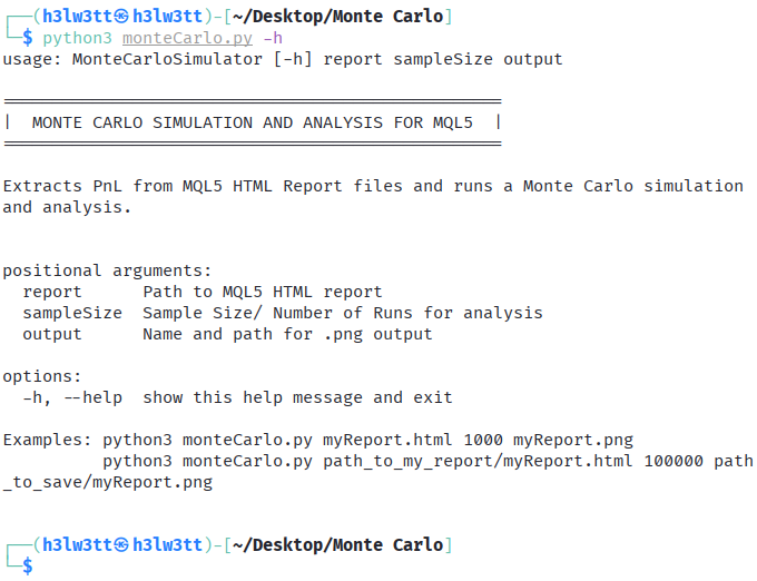
The 'formatter_class' enables us to make the description appear as raw text and place stuff like an ASCII banner and describe what our program does using plain text, and as shown, the epilog places the examples at the end of the help menu. The arguments required are added using the 'add_argument()' call, where we can declare and describe the parameters we need when the program is run from the CLI. The last section ,'args = parser.parse_args()' ,is used to store the values of the arguments input by the user on the CLI, which the program can later on reference and use.

This code is majorly used to run different files easily and for general user-friendliness. One could definitely hard code a file and sample size as well as output file name and location and change it as needed, but that gets old and tiresome, trust me.

Next, data extraction from the HTML report file:

# Read the HTML report
table = pd.read_html(args.report, header=None, match="Deals")[1]

# Find where the Deals section starts
deals_start = table[table
                .astype(str)
                .apply(lambda r: r.str.contains("Deals", case=False, na=False)
                .any(), axis=1)
                ].index[0]

# Use the Deals header row as column names
headers = table.iloc[deals_start + 1]
deals = table.iloc[deals_start + 2:].copy()
deals.columns = headers

# Extract Profit for closed ("out") deals
pnl = (
    deals
    .loc[deals["Direction"].astype(str).str.strip().str.lower() == "out", "Profit"]
    .astype(str)
    .str.replace(" ", "", regex=False)                                                      #Remove thousands separator
    .astype(float)
    .tolist()
)

#Obtain initial balance
initial_balance = 0
balance_row = deals.loc[deals["Type"].astype(str).str.strip().str.lower() == "balance"]

if not balance_row.empty:
    initial_balance = (
        balance_row["Balance"]
        .astype(str)
        .str.replace(" ", "", regex=False)
        .astype(float)
        .iloc[0]
    )
else:
    print("Initial Balance Not Available!")

pnl_df = pd.DataFrame({"PnL": pnl})                                                         #Save the PnL data in a dataframe

This code will be familiar if you have scraped data from websites. Otherwise, a few details below will clarify what happens. The first line of code reads the HTML file and by using pandas, we can obtain the tables in the specified HTML file, and we are specifically looking for tables with the word "Deals" in them. The keen-eyed will notice the '[1]' at the end of the line. This is used to tell pandas that we want the second table, 0 being the first in case anyone is confused with the indexing. Why the second table you may ask? It's because in a MetaTrader 5 report File, the word "deals" appears in two different tables, the first being the list of statistics at the top (Total Deals) and the second being the Orders and Deals table. We want the second table since that contains the data we need.

We then feed the 'deals_start' variable with the index of where the deals data begins. We need to do this since the trade orders and trade deals are combined in one table in the HTML file, so this line of code finds where the 'deals table' begins.

The next three lines locate the headers for the table and the data, and sets the headers as the column headers in the pandas DataFrame for processing the data. After all, we need to know what data means what in the table.

After arranging the data, we proceed to extracting the profit and loss (PnL) data. Here, we filter the data according to the 'Direction' column, where we specify that we want the 'Profit' value (which is our PnL data) if the 'Direction' column contains the value 'out'. This is because Direction = out indicates a closed trade; its profit or loss is stored in the Profit column on the same row.

The next few lines are used to extract the initial balance value, which is conveniently stored on the deals table on the first 'Balance' column entry, but just to be specific, the 'Type' column on the same row contains the word "Balance", so we use that as a filter. The initial balance will be useful for our test since we need a start point for our test, and for compatibility with different files, we need to dynamically extract it so that we don't need to declare it every single time which can lead to grave errors.

We then set the 'initial_balance' variable and also print out an error message if its not set, and package the extracted PnL data to a pandas dataframe so that we can use it for the next step.

With the data in hand, we can proceed to code the Monte Carlo simulation code:

######################(MONTE CARLO MODULE)########################
trades = pnl_df
numberOfTrades = len(trades)-1

allEquityLines = []                                                                        #Stores equity curve data for further analysis
allDrawDowns = []

def MonteCarlo(Trades, initialBalance, No):
        global bust                                                                        #Bust rate variable
        global profit                                                                      #Profit rate variable
        
        peakEquity = initial_balance                                                       #Peak Equity for max drawdown calculation
        maxDraw = 0                                                                        #Max drawdown variable
        equity = initialBalance
        
        rNumbers = random.sample(range(0, No), No)                                         #Creates a random order of indexes based on number of trades
        eY = []                                                                            #Used to store equity values as the simulations occur
        
        for numbers in rNumbers:                                                           #Runs the simulation of an equity curve
                if equity <= 0:
                        equity = 0
                        eY.append(equity)
                        maxDraw = initialBalance
                else:
                        equity += round(Trades.iat[numbers, 0],2)                          #Add the PnL value to the equity after rounding it off
                        eY.append(equity)
                        
                        if equity > peakEquity:                                            #Updates peak equity variable
                                peakEquity = equity
                                
                        drawdown = peakEquity - equity                                     #Calculates current drawdown
                        
                        if drawdown > maxDraw:                                             #Updates max drawdown variable               
                                maxDraw = drawdown
                        
        
        allEquityLines.append(eY)                                                          #Stores the equity curve data of the given run
        plt.plot(eY, alpha = 0.25)                                                         #Plots the equity curve
        
        allDrawDowns.append(maxDraw)                                                       #Store the max drawdown of the run
        
        #Update profit and bust variables
        if equity > initialBalance:
                profit += 1
        elif equity <= 0:
                bust += 1

This is the main part of our code since it is responsible for the generation of the random equity curves. After setting up a few variables and arrays, the first action done by the above code is 'rNumbers = random.sample(range(0, No), No)'. Here, random generates a shuffled order of trade indexes from 0 to the total number of trades. This index is then used to obtain the PnL data it indexes in the 'Trades' dataframe, as shown in the 'for' loop when equity is not less or equal to 0. That filter, the one for checking if equity is less or equals to 0, is necessary so that we don't waste computing power to process an equity curve that is already below zero. Another advantage of this filter is to get rid of false positives since theoretically, an equity curve can come from below zero and end up profitable, which is not practical in real life.

In the 'for' loop, which by now I hope you can see that it is the system that generates the equity curve, we also set the 'maxDraw' parameter which will be useful for analysis later on as it will contain the maximum observed drawdown for our test, a handy statistic.

The code then proceeds to plot the equity lines after storing them in the 'allEquityLines' array that will be used for analysis later on, then storage of the maximum observed drawdown of the run is done and the profit and bust variables are updated.

Next, execution of the Monte Carlo simulation:

x = 0                                                                                      #Sample Size counter
bust = 0                                                                                   #Bust rate variable
profit = 0                                                                                 #Profit rate variable
sampleSize = args.sampleSize                                                               #Sample size variable

#Monte Carlo simulation
while x < sampleSize:                                                                      
        MonteCarlo(trades, initial_balance, numberOfTrades)                                #Generates equity curve
        x += 1                                                                             #increases sample size counter

The sample size parameter enables the creation of multiple equity curves. The larger the number, the more equity curves shall be created and in some scenarios, the better the statistical data extracted.

With the simulation conducted, it is time to see it visually and analyze it:

#Monte Carlo Analysis
allEquityLines = np.array(allEquityLines)                                                  #Stores all equity curve data into an array for further calculation
meanLine = np.mean(allEquityLines, axis = 0)                                               #Calculate the mean equity curve
lowerBand = np.percentile(allEquityLines, 5, axis = 0)                                     #Calculates the lower band for outlier identification
upperBand = np.percentile(allEquityLines, 95, axis = 0)                                    #Calculates the upper band for outlier identification

plt.plot(meanLine, color = "red", linewidth = 3, label = "Mean Equity")                    #Plots mean equity curve
plt.fill_between(                                                                          #Fill the non-outlier range
        range(len(meanLine)), 
        lowerBand, 
        upperBand, 
        alpha = 0.5, 
        color = "gray", 
        label="5-95% Range"
)
plt.xlabel("Trade Number")
plt.ylabel("Equity Curve")
plt.title(args.report)

plt.axhline(y = (initial_balance * 0.5),                                                  #50% drawdown line
        color = "red", 
        linestyle = "--", 
        label = "50% Drawdown"
)
plt.axhline(y = initial_balance,                                                          #Starting balance line
        color="black", 
        linestyle = "--", 
        label="Starting Balance"
)
plt.legend()                                                                              #Display legend
plt.savefig(args.output)                                                                  #Saves the generated image
#plt.show()                                                                               #Definitive edition

maxDrawdown = max(allDrawDowns)                                                           #Obtains the max drawdown observed in the simulation

#Statistics
print("Bust Rate (%): ", (bust/sampleSize) * 100)                                         #Bust Rate    
print("Profit Rate (%): ", (profit/sampleSize) * 100)                                     #Profit Rate
print("Max Drawdown ($): ", round(maxDrawdown,2))                                         #Max Drawdown

gc.collect()                                                                              #Garbage Collection

Numpy finally makes an entrance by storing all the equity curves in an array for the next step, calculating the mean equity curve, as well as the 5th and 95th percentile equity curve. The last two are used to indicate what is normal performance for the strategy and outside these boundaries lie outliers, the abnormal but very possible scenarios in terms of performance of the strategy. 

The code proceeds to outline them on the plot by making the mean line red and thicker as well as indicating it on the legend, and for the 5th and 95th percentile lines, the area between them is colored gray to indicate the 'normal' zone. The next few lines are for labeling various levels of the plot as well as making the legend visible ('plt.legend()' line) and saving the generated plot or displaying it on a different window. I address this in the 'Extra Feature for the statisticians' below.

The last section is mainly for data output to the CLI, starting by getting the maximum observed drawdown and displaying the bust rate, profit rate and max drawdown. Gc then cleans up so that we avoid memory leaks if we were to run multiple instances of this program back-to-back.

With this last bit of code, we are ready to test the program.

Does it work?

Using a test file I had laying around, I run the program with the file placed in the same folder as the program file, and first ran it with a sample size of 100.

Here is the execution line as well as the results:

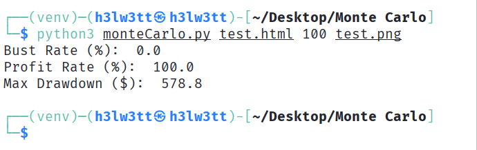
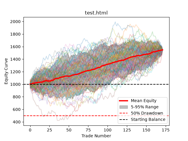
The statistics extracted from this are simple but you can use this program as a baseline to extract way more data from your tests, from longest losing streaks to probability of doubling your account before getting a 50% drawdown.

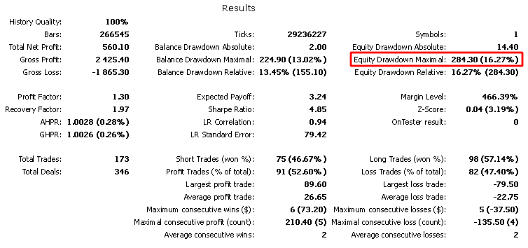
This is the main advantage of Monte Carlo simulation and analysis, obtaining data from a strategy that would otherwise be unknown or misrepresented. In the example above, the simulation shows drawdowns up to $578.80. The original single equity curve in test.html shows only about $284.30, which can lead to underestimating risk and increasing the chance of account blow-up.

As a proof of concept, I forward tested this strategy on out-of-sample data with the same lot size (0.1) which by now, if it isn't evident, is a bit too much as we can experience more than a 50% drawdown indicated by the Monte Carlo simulation and analysis. The results speak for themselves:

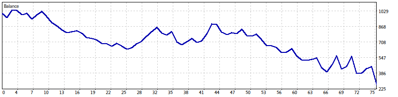
I then went ahead and did this forward test, changing the lot size to 0.01 to simulate a trader who took the information from the Monte Carlo simulation and analysis and adjusted their risk allocation to this strategy. It should also be clear using the above results that we stumbled upon an outlier event in the forward test, where the strategy's performance was critically low for that period of time. But unlike our previous trader who almost went bust, our informed trader's performance tells a different tale:

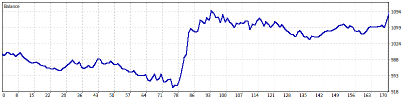
We clearly witness the same poor performance in the beginning of the test but since the informed trader scaled down the risk they took, they were able to come back net positive without going bust. The strategy, despite having quite volatile returns, needs good risk management to be able to rake its positive returns, and with the Monte Carlo system we have developed in this article, such a strategy can be planned for accordingly. 

Other advantages of using the Monte Carlo simulation and analysis system include:

Standard Testing	Standard + Monte Carlo Testing
Single equity curve which leads to one set of data for a strategy	Multiple equity curves that provide a general distribution of data for a strategy
Limited in terms of parameters one can extract from data	Easily customizable to obtain various data parameters such as mean equity and median drawdown
Can lead to extreme risk exposure of a strategy to the market	Curbs excessive risk exposure of a strategy by exposing outlier equity curves

Extra feature for the statisticians

If you would like to see some more statistics on the chart as well as better resolution, you can change the line:

plt.savefig(args.output)                                                                  #Saves the generated image

to:

plt.show()                                                                                #Definitive edition

This opens the graph in a window that enables you to see the X and Y values at any given point on the graph, zoom in and out on any area of the graph and save it just like the original version of the program.

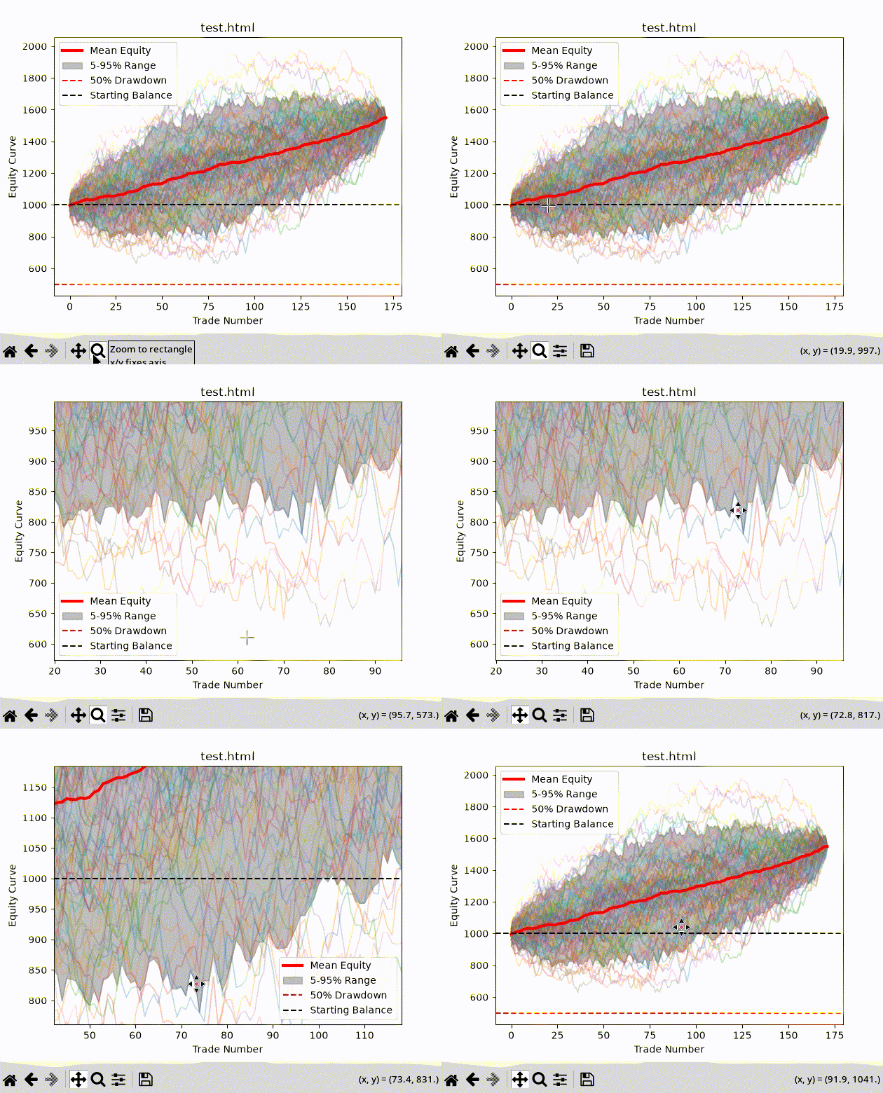
The disadvantage for running the program with this line present is that for low-end PCs as well as denser simulations in terms of number of trades and sample size, it gets quite jittery and resource intensive. The source code contains both lines but the ‘plt.show()’ is commented out for compatibility, but the power is available for all that need it.

Conclusion

Monte Carlo simulation and analysis turn one deterministic backtest into a distribution of realistic outcomes. By extracting closed-trade PnL from an MetaTrader 5 HTML report and running many shuffled simulations, you obtain measurable deliverables — a saved chart with the mean equity and 5–95% range, plus practical statistics (bust rate, profit rate, max observed drawdown). These outputs let you assess the probability of extreme losses, set safer position sizes, and decide whether a strategy needs further refinement or should be discarded.

Use the provided Python script as a starting point: run it on both in-sample and out-of-sample reports, compare the distributions, and adjust risk management based on the simulated tails. Finally, treat the results as a decision-making aid (not a guarantee): expand the analysis if needed (longest losing streaks, time-to-drawdown, etc.) to better match your trading objectives and risk tolerance.