Persistence Entropy as a Market Regime Indicator in MQL5

Contents

1. Introduction: From a Verified Pipeline to a Live Reading
2. The Indicator on a Chart
3. Persistence Entropy
4. Reading H0 and H1 Entropy
5. Loop Strength and the Regime Band
6. The Sliding-Window Engine
7. The Signal Layer
8. Parameter Tuning
9. Live Market Examples
10. Reading the Indicator from an EA
11. Conclusion

Introduction: From a Verified Pipeline to a Live Reading

The previous article finished the engine. A single Compute call now turns a price window into a persistence diagram, and the numbers were checked against an independent reference. We treat that pipeline as a black box here: it produces correct persistence diagrams, and this article puts them to work.

A diagram per window is still a static object. To use it on a live chart you have to solve three concrete problems. First, each diagram must be reduced to a few numbers that update bar by bar. Second, the reduction runs the full O(N^3) pipeline inside OnCalculate. It must not freeze the chart thread. Third, any value derived from a rolling history must be reproducible: the same bar should read the same way no matter how much history happens to be loaded.

To solve all three, the indicator uses a small set of per-bar buffers. They are computed on a sliding window of N closes. Two buffers hold the persistence entropy of dimensions H0 and H1. The rest hold a normalized loop-strength value, a regime code, a z-score, and a signal flag. The window length N (default 80), the maximum simplex dimension (2), and the Vietoris-Rips cutoff are fixed as in the earlier articles. The only new design work here is the rolling layer.

The indicator that produces these buffers is PersistenceEntropy_Indicator. It plots the two entropy lines in a separate window and stamps a small arrow on the main chart when loop-strength enters its high band and price reaches an extreme. This article is a walkthrough of that indicator. It shows how a topological reading of a window becomes a chart object you can read by eye or from code.

This installment assumes the earlier three articles. The Takens embedding and the distance matrix come from the first, the Vietoris-Rips filtration and the boundary matrix from the second, and the reduction, the diagram, and the facade from the third. None of that pipeline is reopened here. All work is in the layer that calls the facade once per window. It converts the output into chart-visible values and EA-readable buffers.

The Indicator on a Chart

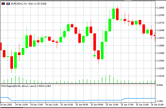
Fig. 1. The indicator on a live chart. The lower window holds the H1 and H0 persistence-entropy lines. The arrows on the main chart mark the fade events described later.

The figure above is the finished product. The lower window carries two lines, the H1 persistence entropy and the H0 persistence entropy, each computed from the persistence diagram of the last N closes. The arrows on the price pane mark the moments where the loop-strength regime is high and price has just stretched to an extreme of its window.

Everything in that picture comes from the same Compute call the series has been building toward. The lines are two scalars pulled from each diagram. The arrows are a small decision layer on top of a third scalar. That is what this article delivers. The rest explains how each number is produced and how the indicator stays responsive while doing it.

Persistence Entropy

A persistence diagram in one dimension is a set of bars, each with a birth and a death. The length of a bar is its persistence, death minus birth. Persistence entropy compresses the whole set of lengths into one number that measures how evenly the total persistence is spread across the bars.

Let the finite bars in a dimension have lengths l_1, l_2, and so on, and let L be their sum. Treat each normalized length as a probability and take the Shannon entropy.

H = -sum_i (p_i) log(p_i), where p_i = l_i / L and L = sum_i l_i

The reading is direct. When one bar dominates and the rest are tiny, the distribution is concentrated and the entropy is low. When many bars share similar lengths, the distribution is flat and the entropy is high. A single clean loop gives low H1 entropy. A scatter of short-lived loops of similar size gives high H1 entropy. The facade computes this directly from the diagram.

//+------------------------------------------------------------------+
//| Persistence entropy of all finite bars in given dimension        |
//|                                                                  |
//|  H_d = -sum (l_i / L) * log(l_i / L)                             |
//|  where l_i = death - birth (finite pairs only) and L = sum l_i.  |
//|  Returns 0 if no finite bars or single bar exists in that dim.   |
//+------------------------------------------------------------------+
double CTDA::PersistenceEntropy(int dim) const
  {
   SPersistencePair pairs[];
   m_diagram.GetByDim(dim, pairs);
   int n = ArraySize(pairs);
   if(n == 0) return 0.0;

   double total = 0.0;
   for(int i = 0; i < n; i++)
     {
      if(pairs[i].IsInfinite()) continue;
      double l = pairs[i].death - pairs[i].birth;
      if(l > 0.0) total += l;
     }
   if(total <= 0.0) return 0.0;

   double H = 0.0;
   for(int i = 0; i < n; i++)
     {
      if(pairs[i].IsInfinite()) continue;
      double l = pairs[i].death - pairs[i].birth;
      if(l <= 0.0) continue;
      double p = l / total;
      H -= p * MathLog(p);
     }
   return H;
  }

The method runs two passes over the finite bars. The first pass sums the lengths to get L. Infinite (essential) bars are skipped, since they have no finite length to contribute. The second pass accumulates the entropy term for each normalized length. Zero-length bars are skipped because they carry no information and their logarithm is undefined. The result is a single non-negative number per dimension.

Two properties make the number easy to read. It is always non-negative, and it is bounded above by the logarithm of the bar count. A window with k equally long bars reaches the maximum, log(k), because the lengths are perfectly even. A window whose total persistence sits in one bar sits near the minimum, close to zero. Between these extremes the value changes smoothly. Rising entropy means persistence spreads across more features; falling entropy means it concentrates into fewer.

A small example fixes the idea. Suppose a window has three H1 bars of length 0.90, 0.05, and 0.05. The total is 1.0, so the probabilities are 0.90, 0.05, and 0.05, and the entropy is about 0.39. Now suppose the three bars are 0.34, 0.33, and 0.33. The total is still 1.0, but the entropy rises to about 1.10, which is close to the maximum of log(3). Same number of loops, same total persistence, very different entropy. The first window has one dominant cycle, the second has three of equal weight.

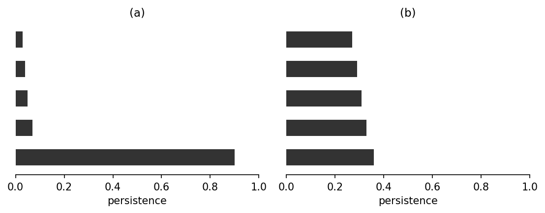
Fig. 2. Two barcodes with the same total persistence. One long bar gives low entropy. Many similar bars give high entropy.

Reading H0 and H1 Entropy

The indicator plots two entropy lines because H0 and H1 measure different things. They are not two views of one quantity. Each answers a separate question about the window.

H0 entropy describes the connected components, which are the merge events of the point cloud. A window where points join into one cluster at a single dominant scale has concentrated H0 lengths and low H0 entropy. A window where merges happen across many different scales has spread-out H0 lengths and high H0 entropy. In market terms, low H0 entropy points to a window that consolidates at one characteristic scale, and high H0 entropy points to fragmented structure with no single scale of organization.

H1 entropy describes the loops. A loop in the embedded cloud is a cyclical pattern in the price window. One dominant loop with a few short ones gives low H1 entropy, the signature of a single clear cycle. Many loops of similar length give high H1 entropy, the signature of tangled, multi-scale cyclical activity. H1 entropy is therefore a measure of cyclical complexity, while H0 entropy is a measure of how the window fragments.

Plotting both keeps the two readings separate. The lines often move independently, and that independence is the point: a window can be cleanly connected yet cyclically complex, or fragmented yet dominated by a single loop.

In practice you watch the two lines for divergence. When H0 entropy falls while H1 entropy stays high, the window is settling into a single connected scale but still carries tangled cyclical activity, a common picture inside a choppy range. When H1 entropy falls while H0 entropy stays high, a single cycle is emerging out of fragmented structure, which often accompanies the early part of a directional move. The absolute levels matter less than the direction each line is moving and whether the two agree or split.

Loop Strength and the Regime Band

Entropy measures the shape of the whole bar distribution. The arrows on the chart use a simpler scalar that measures one thing: how strong the single most persistent loop is, relative to the size of the cloud. We call it loop strength.

loopStr = MaxPersistence(H1) / MaxFiltration

The numerator is the length of the longest H1 bar, the most persistent loop in the window. The denominator is the largest filtration value in the complex, which is the diameter of the cloud at the chosen cutoff. Dividing one by the other removes the price scale, so loop strength is a dimensionless number that is comparable across symbols and time. A value near zero means no loop stands out. A larger value means one cycle dominates the window.

The normalization is what makes the number portable. The raw longest-loop persistence is measured in the same units as the embedded prices, so it grows with volatility and differs across symbols. Dividing by the cloud diameter cancels that scale. A loop strength of 0.4 means the dominant loop spans roughly forty percent of the whole cloud, whether the instrument is a four- or five-digit FX quote or a multi-thousand-point index. That is the property the regime band relies on.

A raw loop-strength number is hard to threshold, because what counts as high depends on the instrument and the period. The indicator solves this by ranking, not by a fixed cutoff. It keeps a rolling history of loop-strength values and classifies the current value against the percentiles of that history. Above the high percentile is REGIME_HIGH, below the low percentile is REGIME_LOW, and the middle is REGIME_MID.

Ranking has a second benefit over a fixed cutoff. It adapts to the instrument on its own. A symbol that rarely forms strong loops still produces a high band, just at a lower absolute value, because the band is defined by the symbol's own recent distribution. A fixed threshold would mislabel a quiet instrument as never high and a wild one as always high. The percentile band sidesteps both by asking a relative question: is this window's loop strength large compared to its own recent past?

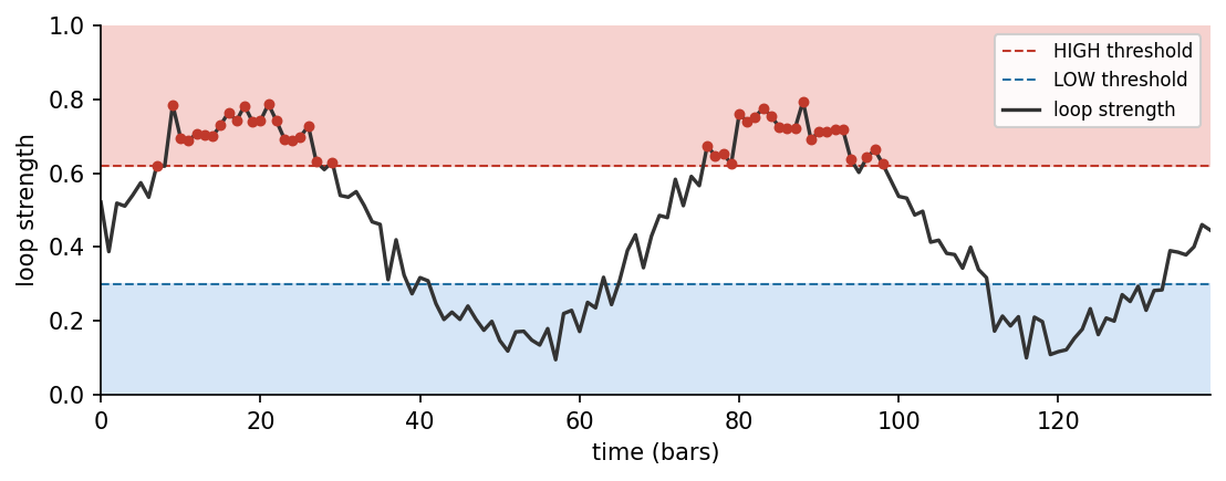
Fig. 3. Loop strength over time against its adaptive percentile band. Values above the high band place the window in REGIME_HIGH.

         if(g_tda.Compute(window, InpWindow))
          {
           BufH0[i] = g_tda.PersistenceEntropy(0);
           BufH1[i] = (InpMaxDim >= 2 ? g_tda.PersistenceEntropy(1) : 0.0);

           double maxFilt = g_tda.MaxFiltration();
           double loopStr = (maxFilt > 0.0 ? g_tda.MaxPersistence(1) / maxFilt : 0.0);

           //--- bands from history before adding the current sample
           double hiCut = PercentileOfHist(InpHighPct, InpRankLookback);
           double loCut = PercentileOfHist(InpLowPct,  InpRankLookback);

           double regime = REGIME_MID;
           if(hiCut > 0.0)
             {
              if(loopStr >= hiCut)            regime = REGIME_HIGH;
              else if(loCut > 0.0 && loopStr <= loCut) regime = REGIME_LOW;
            }

           BufLoopStr[i] = loopStr;
           BufRegime[i]  = regime;
           PushLoopStr(loopStr);
          }

The block computes both entropies, then the loop strength, then the band. The bands are read from the history before the current value is pushed, so the classification is causal: the current sample is never used to set its own threshold. The PushLoopStr call appends the new value with the amortized capacity-doubling pattern introduced in the first article.

The percentile lookup is where reproducibility is enforced. It requires a full reference window before it returns a band at all.

//+------------------------------------------------------------------+
//| Value at percentile p of the last 'lookback' grid samples.       |
//| Requires the full reference window to be present, so the band is |
//| the same set of bars on every reload regardless of how much      |
//| history is loaded. Returns -1 until the window has warmed up.    |
//+------------------------------------------------------------------+
double PercentileOfHist(double p, int lookback)
  {
   int avail = g_lsCount;
   if(avail < lookback) return -1.0;

   double tmp[];
   ArrayResize(tmp, lookback);
   int from = avail - lookback;
   for(int i = 0; i < lookback; i++) tmp[i] = g_lsHist[from + i];
   ArraySort(tmp);

   int idx = (int)MathRound(p * (lookback - 1));
   if(idx < 0)           idx = 0;
   if(idx > lookback - 1) idx = lookback - 1;
   return tmp[idx];
  }

If fewer than lookback samples exist, the function returns -1 and the regime stays REGIME_MID, so no signal can fire. Once the history is warmed up, the band is always read from exactly the last lookback samples, which are the same set of bars on every reload. This is the property that matters in practice. With less history loaded the indicator simply emits no arrows for the un-warmed region, rather than emitting different arrows. Either you have enough history and the marks are reproducible, or you do not have enough and there are no marks. The marks never change for a given bar between reloads.

The cost of this guarantee is the warm-up. Until the reference window is full, the indicator shows its entropy lines but draws no marks. That is a deliberate trade. If a mark changes meaning depending on loaded history, it is better to show no mark. Requiring a full window keeps the marks honest at the price of a quiet start.

The Sliding-Window Engine

The full pipeline is expensive. Each window runs the embedding, the distance matrix, the filtration, the boundary, the reduction, and the diagram, and the cost grows with the cube of the point count. Recomputing that on every historical bar at first attach would block the chart thread and look frozen. Two guards keep the indicator responsive.

Fig. 4. Each window flows through one Compute call to a diagram, then to the scalars that fill the buffers.

The first guard is a history cap. On first load the indicator computes only the last InpHistoryBars bars and writes EMPTY_VALUE to the plotted buffers before that point. A heavy recomputation across thousands of bars is what makes a chart freeze, and the cap bounds that one-time cost. The second guard is a step grid. The heavy Compute runs only on bars whose index is a multiple of InpStep, and the lines hold their last value between grid points.

      //--- heavy TDA only on the step grid; the lines hold between grid points
      bool gridBar = ((i % step) == 0) || (i == rates_total - 1);

Neighboring windows overlap by all but one bar, so their diagrams barely differ. Computing every tenth window and holding the value in between gives a smooth, continuous plot at a fraction of the cost. The last bar is always treated as a grid bar so the most recent reading is current. InpStep is the direct tradeoff between responsiveness and update granularity: a larger step is faster but updates the lines less often.

The z-score of the latest close is cheap, so it is computed on every bar regardless of the grid. That keeps the extreme detection sharp even between heavy recomputations. The regime and entropy values come from the grid and are held steady until the next grid bar.

There is one more guard at the top of OnCalculate. Between ticks of the same bar the closed history does not change, so a tick that arrives with no new bar returns immediately. Recomputing topology on every incoming tick would be wasteful, since the entropy of a set of closed bars is fixed until a new bar forms. The indicator computes on bar boundaries, not on ticks.

On first load the buffers before the computed region are cleared. The plotted lines get EMPTY_VALUE, and the calculation buffers get neutral values. This keeps the plot clean and gives any reader a defined value even in the un-warmed region. The clearing loop runs once, and from then on the indicator only extends the most recent bars.

The Signal Layer

The arrows combine two conditions: price has just reached an extreme of its own window, and the loop-strength regime is high. The extreme is measured by a z-score of the latest close inside its window, using a small helper that returns the window mean and standard deviation.

      //--- z-score of the latest close inside its window (cheap, every bar)
      double mean, sd;
      MeanStd(close, base, i, mean, sd);
      double z = (sd > 0.0 ? (close[i] - mean) / sd : 0.0);
      BufZ[i] = z;

The z-score is deliberately local to the window. It measures how far the latest close sits from the mean of the same N bars the topology is computed on, in units of that window's standard deviation. A close two standard deviations above its window mean is a genuine stretch relative to recent behavior, regardless of the absolute price. Tying the extreme test to the same window as the diagram keeps both halves of the signal on the same footing.

A signal should fire on the bar that first enters the extreme, not on every bar that stays there. The indicator compares the current z-score to the previous bar's value. Only a new threshold crossing is treated as an event. Without additional logic, values oscillating around the threshold can re-trigger crossings on nearby bars. This produces clusters of arrows on a single move. A hysteresis latch prevents that.

      //--- hysteresis latch: after a fade signal the price must return toward
      //    the mean (abs z < InpZReset) once before a new signal is allowed.
      bool armed = true;
      for(int j = i - 1; j >= base; j--)
        {
         if(BufSignal[j] != 0.0)
           {
           armed = false;
           for(int k = j + 1; k < i; k++)
              if(MathAbs(BufZ[k]) < InpZReset) { armed = true; break; }
           break;
         }
        }

      //--- fade signal: fresh excursion while the held regime is HIGH
      double sig = 0.0;
      if(crossing && armed && BufRegime[i] == REGIME_HIGH)
         sig = (z > 0.0 ? -1.0 : 1.0);      // above the mean: sell, below: buy
      BufSignal[i] = sig;

      if(sig != 0.0 && i < rates_total - 1)
         DrawArrow(time[i], (sig > 0.0 ? low[i] : high[i]), sig > 0.0);

The latch scans back through the current window for the most recent signal. If one exists, a new signal is blocked until the z-score has dipped back below the reset threshold at least once. The scan reads the signal and z-score buffers, so it stays consistent through recomputes and never looks ahead. The fade direction is the opposite of the excursion: an extreme above the mean produces a down mark, an extreme below produces an up mark. The arrow is drawn only on closed bars, so the live bar never paints a mark that later disappears.

The marks themselves are simple chart objects.

//+------------------------------------------------------------------+
//| Drop a fade arrow on the main chart window                       |
//+------------------------------------------------------------------+
void DrawArrow(datetime t, double price, bool buy)
  {
   if(!InpDrawArrows) return;
   string name = g_arrowPrefix + IntegerToString((long)t);
   if(ObjectFind(0, name) >= 0) return;
   ObjectCreate(0, name, OBJ_ARROW, 0, t, price);
   ObjectSetInteger(0, name, OBJPROP_ARROWCODE, buy ? 233 : 234);
   ObjectSetInteger(0, name, OBJPROP_COLOR, buy ? clrLime : clrRed);
   ObjectSetInteger(0, name, OBJPROP_WIDTH, 1);
   ObjectSetInteger(0, name, OBJPROP_ANCHOR, buy ? ANCHOR_TOP : ANCHOR_BOTTOM);
  }

Each arrow is named using the bar timestamp, so it is created once and never duplicated. The up mark is drawn below the bar and the down mark above it, which keeps the marks clear of the candles. The object prefix lets the indicator remove only its own arrows when it is detached.

One detail keeps the marks trustworthy. The signal is evaluated and the arrow drawn only for closed bars, never for the bar still forming. A mark, once placed, does not move or vanish on the next tick. The hysteresis scan reads decisions already written to the buffers rather than recomputing them, so the marks stay stable across recomputations and chart reloads.

Six buffers carry the full reading. Two are plotted lines, and four are calculation buffers that an EA can read.

Buffer	Name	Contents
0	PE H1	H1 persistence entropy (plotted)
1	PE H0	H0 persistence entropy (plotted)
2	LoopStr	loop-strength value
3	Regime	0 = REGIME_LOW, 1 = REGIME_MID, 2 = REGIME_HIGH
4	Signal	+1 buy-fade, -1 sell-fade, 0 none
5	ZScore	window z-score of the last close

Parameter Tuning

The indicator exposes the engine settings from the earlier articles plus the new signal-layer controls. The defaults are a sensible starting point. The table lists the parameters most worth adjusting and what each one trades off.

//--- inputs: engine
input int           InpWindow      = 80;                 // sliding window length
input int           InpEmbDim      = 3;                  // embedding dimension
input int           InpDelay       = 1;                  // time delay (tau)
input int           InpMaxDim      = 2;                  // max simplex dim (1 = H0 only, 2 = H0+H1)
input double        InpMaxEpsFrac  = 0.5;                // VR epsilon cutoff = fraction of max pairwise distance
input ENUM_TDA_NORM InpNorm        = TDA_NORM_EUCLIDEAN; // distance norm
input bool          InpUseLog      = false;              // use log-returns instead of raw close

//--- inputs: signal layer
input double        InpZEntry      = 1.0;                // price extreme threshold (abs z-score)
input double        InpZReset      = 0.5;                // re-arm threshold: abs z must dip below this first
input int           InpRankLookback= 30;                 // grid samples in the band reference window (warm-up)
input double        InpHighPct     = 0.667;              // percentile for the HIGH threshold
input double        InpLowPct      = 0.333;              // percentile for the LOW threshold

//--- inputs: performance and display
input int           InpStep        = 10;                 // recompute every N bars (>= 1)
input int           InpHistoryBars = 800;                // bars of history on first load (0 = all)
input bool          InpDrawArrows  = true;               // draw fade arrows on the main chart

Parameter	Typical range	Effect
InpWindow	60 to 120	Larger windows see longer structure but cost more and react slower
InpEmbDim	2 to 4	Higher dimension unfolds more structure at higher cost
InpDelay	1 to 3	Spacing between lagged samples in the embedding
InpMaxEpsFrac	0.4 to 1.0	VR cutoff as a fraction of cloud diameter; lower is faster, higher sees more loops
InpStep	5 to 20	Recompute cadence; higher is faster but updates the lines less often
InpHistoryBars	500 to 2000	History computed on first load; larger covers more chart but takes longer to warm up
InpRankLookback	20 to 60	Reference window for the regime band; sets the warm-up length
InpZEntry	1.0 to 2.0	How far price must stretch before a mark can appear

The relationship between InpRankLookback, InpStep, and InpHistoryBars is worth stating plainly. The band needs InpRankLookback grid samples to warm up, and each grid sample is InpStep bars apart. So the warm-up consumes about InpRankLookback times InpStep bars, and InpHistoryBars must be larger than that for any mark to appear. With the defaults the warm-up is about 300 bars, and the marks begin once enough history is loaded.

Live Market Examples

Across different market conditions the indicator behaves as a structural description of the window rather than a forecast. Each condition leaves a distinct fingerprint on the entropy lines and the regime band. The three examples below show the same indicator on a trending, a ranging, and a volatile stretch.

In a trending market price moves persistently in one direction. The embedded cloud stretches into an elongated shape with few closed loops, so loop strength is modest and the H1 entropy is low. H0 entropy is also low, because the points merge along one dominant direction. The regime rarely reaches REGIME_HIGH, so marks are sparse. This is the picture of a window with clear direction and little cyclical structure.

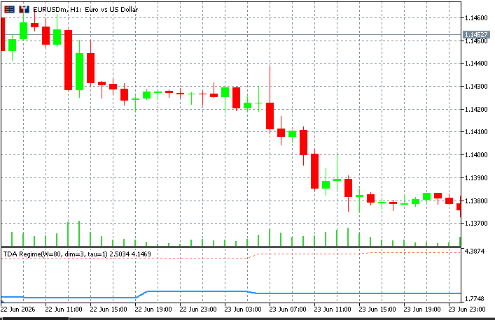
Fig. 5. A trending stretch. Loop strength stays modest and the regime rarely reaches REGIME_HIGH, so marks are sparse.

In a ranging market price oscillates inside a band. The cloud curls back on itself and forms loops, so loop strength rises and the regime reaches REGIME_HIGH more often. The H1 entropy depends on whether one cycle dominates or several compete. This is the condition where the fade marks appear most, because price repeatedly reaches the edges of its window while a strong loop is present.

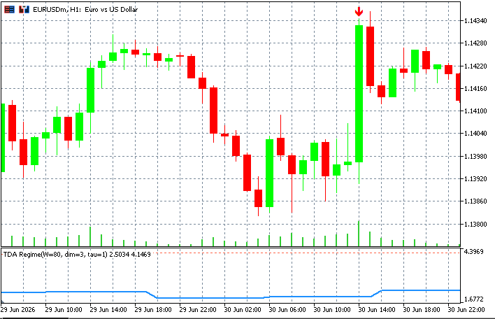
Fig. 6. A ranging stretch. Loop strength rises, the regime reaches REGIME_HIGH, and the fade marks appear at the band edges.

In a volatile market large bars dominate. The cloud is wide and irregular, H0 entropy climbs as merges happen across many scales, and loop strength can spike and collapse quickly. The regime band reacts but the picture is noisier. The reading here is less about marks and more about the entropy lines flagging a window with no clean structure.

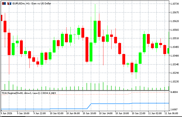
Fig. 7. A volatile stretch. H0 entropy climbs and loop strength spikes and collapses, flagging a window with no clean structure.

Reading the Indicator from an EA

Because the loop-strength, regime, signal, and z-score live in calculation buffers, an Expert Advisor can read them with iCustom and CopyBuffer. The buffer indices match the table above. The indicator is located in the TDA subfolder of Indicators, so the iCustom name is prefixed with TDA followed by an escaped backslash. The sketch below reads the regime code on the last closed bar.

int handle = INVALID_HANDLE;

int OnInit()
  {
   handle = iCustom(_Symbol, _Period, "TDA\\PersistenceEntropy_Indicator");
   if(handle == INVALID_HANDLE)
      return INIT_FAILED;
   return INIT_SUCCEEDED;
  }

void OnTick()
  {
   double regime[];
   if(CopyBuffer(handle, 3, 1, 1, regime) != 1)   // buffer 3 = Regime, last closed bar
      return;

   if(regime[0] == 2.0)
     {
      // window is in the HIGH loop-strength regime
     }
   else if(regime[0] == 0.0)
     {
      // window is in the LOW loop-strength regime
     }
  }

This is a sketch, not a production-ready EA. It shows the mechanics: get the indicator handle once in OnInit, then copy the buffer value you need on each tick. The same pattern reads buffer 0 or 1 for the entropy lines, buffer 2 for loop strength, or buffer 5 for the z-score. Reading the last closed bar (index 1) rather than the forming bar keeps the value stable, since the indicator only marks closed bars. What an EA does with these values is a separate design question, and the indicator stays a descriptive layer that reports the topological reading of the window.

A production reader would do a little more. It would act on new bars rather than every tick, by tracking the last processed bar time and proceeding only when it changes. It would read the entropy and z-score buffers alongside the regime to build a fuller picture of the window. And it would release the indicator handle in OnDeinit. The sketch leaves these out to keep the mechanics visible, but they are the difference between a demonstration and a deployable reader.

Conclusion

This article concludes the series by turning the verified pipeline into a live reading. The indicator runs the full Takens-to-diagram pipeline on a sliding window, reduces each diagram to persistence entropy and loop strength, and exposes the result as plotted lines, chart marks, and EA-readable buffers.

• Persistence entropy summarizes the spread of bar lengths in a dimension. H0 entropy reads as fragmentation, H1 entropy as cyclical complexity.
• Loop strength normalizes the strongest loop by the cloud diameter, and an adaptive percentile band classifies it into REGIME_LOW, REGIME_MID, and REGIME_HIGH.
• A full warm-up window makes the band reproducible: the same bar reads the same way regardless of how much history is loaded.
• A history cap and a step grid keep the heavy O(N^3) pipeline responsive inside OnCalculate.

You can now attach PersistenceEntropy_Indicator, watch the two entropy lines and the regime marks update on closed bars, and read any of the six buffers from an Expert Advisor. The indicator is a descriptive instrument: it reports the topological structure of each window and leaves the interpretation to you.

From here the natural extensions are open. The same pipeline accepts a multivariate embedding for joint analysis of two series. The persistence diagrams can be compared with diagram distances such as the bottleneck or Wasserstein metric, which opens the door to clustering windows by shape. And the regime code is a ready label for a classifier that learns which structural states matter for a given instrument. The library is small, verified, and self-contained, and each of these is a clean next step.

#	Filename	Type	Description
1	TDAPointCloud.mqh	Header	Takens embedding (from Article 1)
2	TDADistance.mqh	Header	Pairwise distance matrix (from Article 1)
3	TDARips.mqh	Header	Vietoris-Rips filtration (from Article 2)
4	TDABoundary.mqh	Header	Boundary matrix over Z/2 (from Article 2)
5	TDAReduction.mqh	Header	Column reduction to persistence pairs (from Article 3)
6	TDADiagram.mqh	Header	Persistence diagram and analytics (from Article 3)
7	TDA.mqh	Header	CTDA facade, full pipeline (from Article 3)
8	PersistenceEntropy_Indicator.mq5	Indicator	Persistence-entropy and regime indicator (this article)