Trust Your Backtest Data First: Building a Reproducible Historical Data Audit in Python for MetaTrader 5

Introduction

Every backtest result inherits the quality of its input data, yet few people check that data before computing statistics. Traders routinely see MetaTrader 5's built‑in “History Quality” drop from 99% to 30% without knowing why. Others discover too late that their feed had silent gaps in the exact period they tested. The forums are full of the same question — "how do I verify my history is complete across several pairs?" — and the usual answer is "write a script yourself."

This article is that script. It builds a reproducible, read‑only data audit that you run once before trusting any backtest. Then it shows why the audit matters by running the same trivial strategy on data from three brokers and measuring the result drift. The brokers are anonymized throughout (Broker A, B, C) — the point is not who is "best," but that "the same backtest" is an illusion the moment the data underneath it changes.

Everything here is reproducible. Full Python source is attached; it imports only read-only functions (API calls) from the MetaTrader 5 package and never touches an order function.

What we are going to build

Three pieces, each a section below:

1. A multi-broker exporter that pulls M5 history per pair from each terminal in read-only mode and caches it as Parquet, so every later run is instant.
2. A gap audit that builds the expected 5-minute grid and classifies every missing bar as benign (weekend, rollover, holiday) or a real defect — reported per pair and per year, not as one global number that hides a bad year.
3. A demonstration: one identical, deterministic strategy run on all three feeds over a common window, with the result difference decomposed into its causes.

Pulling history from three terminals without stepping on yourself

The MetaTrader 5 Python API connects to a running terminal. With several brokers installed, the first risk is connecting to the wrong terminal. Before exporting any bars, the exporter verifies the terminal by path and company name and aborts on a mismatch.

import os
import MetaTrader5 as mt5

# Label -> terminal path + expected company. Verification is primarily by path.
BROKERS = {
    "brokerA": dict(path=r"<PATH-TO-MT5-A>\terminal64.exe", company_hint="Broker A"),
    "brokerB": dict(path=r"<PATH-TO-MT5-B>\terminal64.exe", company_hint="Broker B"),
    "brokerC": dict(path=r"<PATH-TO-MT5-C>\terminal64.exe", company_hint="Broker C"),
}

def same_or_inside(real_path, exe_path):
    """Does the terminal's reported data dir match the expected install path?"""
    exp = os.path.normcase(os.path.normpath(os.path.dirname(exe_path)))
    rp  = os.path.normcase(os.path.normpath(real_path or ""))
    return rp == exp or exp in rp

def export_broker(label, cfg):
    if not mt5.initialize(path=cfg["path"]):          # attach to THIS terminal
        return False

    ti = mt5.terminal_info()
    company, real_path = (ti.company or ""), ti.path

    # SAFETY: with several terminals running, initialize() can attach to the
    # wrong one. Path OR company must match, otherwise abort before any export.
    path_ok = same_or_inside(real_path, cfg["path"])
    hint_ok = cfg["company_hint"].lower() in company.lower()
    if not path_ok and not hint_ok:
        mt5.shutdown()
        raise SystemExit(f"ABORT: '{company}' @ {real_path} != expected {cfg['path']}")

    names = [s.name for s in (mt5.symbols_get() or [])]
    # ... per pair: resolve_symbol(), fetch (range|paged), cache as Parquet ...
    mt5.shutdown()                                    # close before the next broker
    return True

# Strictly ONE broker after another -- never two MT5 connections at once:
for label in ("brokerA", "brokerB", "brokerC"):
    export_broker(label, BROKERS[label])

Two hard rules sit behind this code. First, never run two Python processes against terminals at the same time — the API returns empty results under contention, silently. The export runs strictly one broker after another, with shutdown() in between. Second, the package requires Python 3.12; it does not install on 3.13/3.14 at the time of writing.

Brokers also name their symbols differently — e.g., EURUSD, EURUSD.r, EURUSDm, or a 'p' suffix on crosses only. The resolver maps each broker's real symbol to a canonical pair name, trying an exact match first, then an inverted match, then a suffix match on the first six characters, and documents which real name it used:

CCYS = ["USD", "EUR", "GBP", "JPY", "CHF", "AUD", "NZD", "CAD"]   # 8 -> 28 pairs

def resolve_symbol(base, quote, available):
    """Map a pair to the broker's real symbol, suffix-tolerant.
    Returns (chosen, inverted, candidates)."""
    a, b = base + quote, quote + base
    up = {s.upper(): s for s in available}
    if a in up:                       # exact, e.g. EURUSD
        return up[a], False, [up[a]]
    if b in up:                       # exact inverted: broker quotes quote/base
        return up[b], True, [up[b]]
    fwd, rev = [], []                 # suffix: EURUSD.r / EURUSDm / EURGBPp ...
    for u, orig in up.items():
        if   u[:6] == a: fwd.append(orig)
        elif u[:6] == b: rev.append(orig)
    if fwd: return sorted(fwd, key=len)[0], False, sorted(fwd, key=len)
    if rev: return sorted(rev, key=len)[0], True,  sorted(rev, key=len)
    return None, None, []

Each broker's bars are cached into its own folder ( brokerA/ , brokerB/ , brokerC/ ) as Parquet. Every later run — the audit, the backtest — reads only the cache and never re-touches a terminal.

One broker needed special handling. Its terminal refused large copy_rates_range calls ("Invalid params"), so history had to be pulled by backward paging with copy_rates_from_pos in shrinking chunks. That detour surfaced something worth a whole section of its own — see below.

The audit: telling a holiday from a hole

A gap audit is conceptually simple: build the full expected 5-minute grid from the first to the last bar, and every slot that should exist but doesn't is a gap. The judgment is in classifying those gaps. A missing bar on a Saturday is not a defect; a missing hour on a Tuesday afternoon might be. The daily rollover minute and holidays are benign; a broker simply not having data for a year is not.

FREQ = "5min"

def analyze(t):                          # t = sorted bar timestamps (Series)
    first, last = t.iloc[0], t.iloc[-1]
    grid    = pd.date_range(first, last, freq=FREQ)   # complete target grid
    have    = pd.DatetimeIndex(t.values)
    missing = grid.difference(have)                   # slots that should exist

    wk = missing.weekday
    intraweek = missing[(wk >= 0) & (wk <= 4)]        # Mon-Fri = potential DEFECT
    weekend   = missing[(wk == 5) | (wk == 6)]        # Sat/Sun = closed (benign)

    expected_week = grid[(grid.weekday >= 0) & (grid.weekday <= 4)]
    miss_pct = 100.0 * len(intraweek) / max(len(expected_week), 1)
    return dict(bars=len(t), first=first, last=last,
                miss_pct=miss_pct, weekend=len(weekend))
# Benign: holidays, the midnight rollover (1 slot), summer thin liquidity.
# Defect: wide Mon-Fri holes in the active session, or a whole missing year.
# Reported per pair AND per year -- never as one global percentage.

The key reporting choice is per year, not one global percentage. A single "1.6% missing" number can hide a year that is 40% empty by averaging it against eight clean ones. Broken out by year, a bad patch is obvious at a glance — and that breakdown is what reveals the differences between brokers.

Here is what the same 28-pair, M5 request returned from each of the three terminals:

Broker	Bars	First	Last	All 28 pairs from	Mon - Fri gap
A	42,430,519	2005-01-02	2026-06-12	2006-12-11	5.99%
B	32,334,143	2005-01-03	2026-06-12	2025-01-02	2.23%
C	2,800,000	2025-01-31	2026-06-12	2025-02-07	1.57%

Same request, three very different datasets. Broker A reaches back to 2005 with full pair coverage from late 2006. Broker B reaches back similarly far by total bar count, but seven pairs contain real data only from January 2025. This is a broker limitation, not a bug. A 2015 request returned a single bar despite triggering a download. Broker C holds exactly 100,000 bars per symbol on a rolling window, so its history simply stops around 14 months ago, no matter what you request.

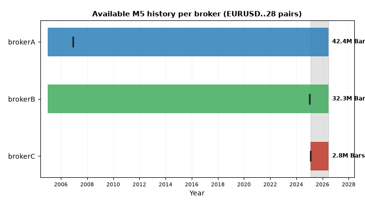
Available M5 history per broker. Broker A and B reach back to 2005 in total, but B's full-pair coverage and C's hard 100,000-bar ceiling shrink the window where all three feeds overlap to roughly 16 months.

Note Broker A's higher gap percentage: it comes entirely from thin pre-2015 crosses across the full depth — benign, and identical to a separate single-broker audit. This is exactly why the per-year breakdown matters: the global number looks worse for A, but the test-relevant years are clean.

A detour worth keeping: when "history" is invented

Broker A's range-based export starts in 2005 and is clean. But the backward-paging method needed for Broker C, when pointed at Broker A's terminal, returned over two million bars reaching back to 1971 — for the euro, which did not exist until 1999.

These early bars are synthetic. The instructive part is how you detect them, because the obvious tests fail:

• Flat OHLC does not work. The very oldest bars are flat (O=H=L=C), but from the early 1970s onward the synthetic daily bars carry a real-looking range. And flat bars also occur legitimately in real M5 data — illiquid 5-minute slots, 0.37% of the real cache. Filter on "flat" and you mislabel real bars.
• Volume does not work: real_volume is 0 throughout forex; tick_volume is only a hint on the very first bars.
• The bar spacing works. The synthetic bars sit in an M5 timeframe but are spaced one day apart (three days over weekends). A 5-minute series with daily timestamps is unambiguously synthetic.

# Core test: an M5 series with DAILY spacing is synthetic (not real 5-minute data).
df["flat"] = (df.open == df.high) & (df.high == df.low) & (df.low == df.close)
df["gap_to_next_min"] = df.dt.shift(-1).sub(df.dt).dt.total_seconds() / 60

per_year = df.groupby(df.dt.dt.year).agg(
    bars          = ("dt", "size"),
    pct_daily_gap = ("gap_to_next_min", lambda s: 100 * (s >= 1440).mean()),  # 1 day
    pct_5min_gap  = ("gap_to_next_min", lambda s: 100 * (s == 5).mean()),     # real M5
)
# Result (Broker A, EURUSD): until 1998 ~255 bars/yr, 100% daily-spaced (synthetic);
# from 1999 ~74,000 bars/yr, ~99% 5-minute (real).
# Flat OHLC alone fails (real quiet bars are flat too); real_volume is 0 across
# forex-useless. The timestamp spacing is the one reliable criterion.

The break is razor-sharp at the euro's introduction: roughly 255 bars per year before 1999 (100% daily-spaced, synthetic), roughly 74,000 per year from 1999 on (99% genuine 5-minute).

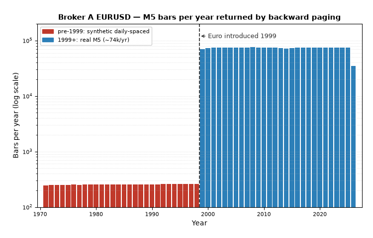
Bars per year returned by backward paging from Broker A. The pre-1999 block is synthetic, daily-spaced data, not real M5 — visible as the sharp jump at the euro's introduction in 1999. The range-based export used for the audit excludes it entirely; the cache starts in 2005 with zero pre-2005 bars.

To be clear about scope: these synthetic bars are not in the backtest cache. The range-based export starts in 2005 and never pages back this far. The lesson is methodological — how you request history partly determines what you get, and the only reliable validator is the timestamp spacing.

The demonstration: one strategy, three feeds

Now the part that makes the audit matter. The question is not "which broker wins" — it is "how much does the same code move when only the data underneath it changes?"

The strategy is deliberately trivial and deterministic, chosen so it has no edge to distract from the comparison: a time-of-day breakout. Take the high and low of the first hour after 08:00 broker time as a reference range; go long on a break above the range high, short on a break below the low; exit at 17:00; one position per day per symbol; no stop, no target. Tested on the three liquid majors (EURUSD, GBPUSD, USDJPY) over the common window 2025-02-07 to 2026-06-12.

Lookahead protection is the same structural guard as in any honest simulator: the signal forms on bar close, the fill is on the next bar's open, and an assertion enforces it on every trade.

RANGE_HOUR, EXIT_HOUR = 8, 17        # range [08:00,09:00); exit first bar >= 17:00

def backtest_symbol(df, pip):
    times = df["time"].to_numpy(); hour = df["time"].dt.hour.to_numpy()
    o, h, l, c = (df[x].to_numpy() for x in ("open", "high", "low", "close"))
    trades = []
    for d, idx in df.groupby(df["time"].dt.normalize()).groups.items():
        idx = np.asarray(idx); hh = hour[idx]
        rng = idx[hh == RANGE_HOUR]; ex = idx[hh >= EXIT_HOUR]
        if len(rng) == 0 or len(ex) == 0: continue
        rng_hi, rng_lo = h[rng].max(), l[rng].min()       # reference range
        exit_i = ex[0]; exit_time, exit_price = times[exit_i], o[exit_i]

        sig_i = direction = None                           # first break in [09:00, exit)
        window = idx[(times[idx] >= d + np.timedelta64(9, "h")) & (times[idx] < exit_time)]
        for i in window:
            if   c[i] > rng_hi: sig_i, direction = i, "long";  break
            elif c[i] < rng_lo: sig_i, direction = i, "short"; break
        if sig_i is None: continue

        entry_i = sig_i + 1                                # fill on the NEXT bar's open
        if entry_i >= len(df): continue
        entry_time, entry_price = times[entry_i], o[entry_i]
        assert entry_time > times[sig_i], "lookahead!"     # guard on every trade
        if entry_time >= exit_time: continue
        gross = ((exit_price - entry_price) if direction == "long"
                 else (entry_price - exit_price)) / pip
        trades.append(dict(date=pd.Timestamp(d), direction=direction, gross_pips=gross))
    return pd.DataFrame(trades)

# net_pips = gross_pips - spread_pips      (spread_pips = spread_pts * point / pip)

# --- Decompose the net difference between two feeds (A - B), per symbol ---
same_dir = common_days[dir_a == dir_b]                          # identical signal
data_price_effect       = (gross_a - gross_b)[same_dir].sum()         # different bars
cost_spread_effect      = -(spread_a - spread_b) * len(same_dir)      # pure spread
different_trades_effect = only_a_net - only_b_net + diff_dir_net      # signal missing/flips
assert round(data_price_effect + cost_spread_effect
             + different_trades_effect, 1) == round(net_a - net_b, 1)  # checksum

The identical code, identical window, identical parameters — run three times, once per feed. Each broker's own spread snapshot is applied, since the spreads differ enormously. Net results, in pips:

Broker / Symbol	Trades	Gross	Net	PF	Win%	Spread
A EURUSD	347	−650.0	−684.7	0.86	49.0	0.1
A GBPUSD	347	23.2	−601.4	0.89	49.0	1.8
A USDJPY	346	−636.1	−1777.9	0.76	44.5	3.3
B EURUSD	349	−830.2	−1318.8	0.75	47.0	1.4
B GBPUSD	349	191.0	−576.8	0.90	49.0	2.2
B USDJPY	348	−1330.8	−1992.0	0.74	46.3	1.9
C EURUSD	349	−807.4	−3634.3	0.45	37.2	8.1
C GBPUSD	349	243.0	−4992.0	0.38	37.2	15.0
C USDJPY	348	−1145.0	−5425.4	0.44	35.6	12.3

The strategy loses on every feed — by design, and beside the point. What matters is the spread between feeds: the same rule drifts by roughly 2,300 to 4,400 net pips depending on the data source, and the profit factor falls from around 0.85 on A and B to around 0.40 on C.

Net result of one identical strategy across three feeds — same window, same parameters, only the data feed differs. The strategy has no edge; the divergence comes entirely from the data and costs underneath it.

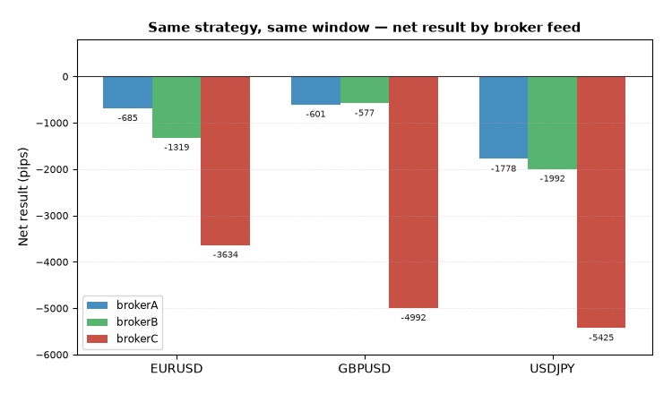
Where the difference comes from

A drift number is only useful if you can decompose it. Each pairwise difference splits cleanly into three causes (a checksum assertion confirms the parts reconstruct the whole exactly): the cost effect (different spreads), the data/price effect (identical signal, but slightly different bars give different entry/exit prices), and the trade effect (missing or differing bars create or suppress signals).

Symbol	Pair	Net diff	data price	cost_spread	diff_trades
EURUSD	A-C	2949.6	−118.8	2648.0	420.4
GBPUSD	A-C	4390.6	−222.6	4342.8	270.4
USDJPY	A-C	3647.5	−246.3	2952.0	941.8
EURUSD	A-B	634.1	−112.2	431.6	314.7
GBPUSD	A-B	−24.6	−213.4	131.2	57.6
USDJPY	A-B	214.1	−160.3	−460.6	835.0

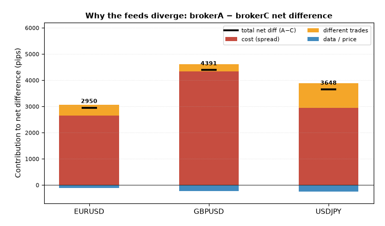
Decomposition of the A−C net difference. The spread (cost) term dominates, but the data/price term (same signal, slightly different bars) and the trade term (missing or flipped signals) are both real and non-zero. No broker is a clean superset of another. The B−C decomposition looks similar.

The spread difference dominates the headline drift. However, the spreads shown are weekend snapshots, not time‑weighted averages. Broker C's 8.1‑pip EURUSD spread is a closed‑market demo value and would be much narrower live. So treat the cost column as an illustration of the spread between feeds, not as a live cost model.

The more interesting findings are the two that survive even if you ignore costs entirely. The data/price effect is small but real: at an identical signal, entry prices differ by 0.6–1.2 pips on average across feeds (with one 47.7-pip USDJPY outlier). And the trade effect is structural: Broker A produces two fewer trade-days per symbol than B and C because of missing bars, and on individual days the brokers even take opposite directions — GBPUSD went the opposite way on 19 of 347 days between A and B alone (EURUSD 15, USDJPY 17). No broker is a clean superset of another.

What to take away

A few things worth keeping, whichever broker you trade:

1. Audit before you compute. Build the expected bar grid, classify gaps as benign or defect, and report per year — a global percentage hides the year that ruins your test. It is the cheapest insurance in all of backtesting.
2. How you request history changes what you get. A range request and a paging request against the same terminal can return different things — including synthetic bars that look real. Validate by timestamp spacing, not by flat OHLC or volume.
3. "The same backtest" is an illusion without the same data. An identical, deterministic strategy drifted by 2,300 to 4,400 pips and halved its profit factor across three feeds. Most of that was cost, but a real, irreducible part was the data itself: different prices at the same signal, and different signals altogether.
4. A negative result is still a result. The strategy here has no edge — that was the point. The value is the method: a reproducible way to answer "Can I trust this data, and does the source change my conclusion?" with evidence instead of hope. Before optimizing a strategy, make sure the history you optimize on deserves your trust.

How to run this yourself (no prior Python experience required)

Everything below is read-only — the code only reads price history out of MetaTrader 5 and never places, modifies, or closes a trade. If you have never used a command line before, the full step-by-step walkthrough (with troubleshooting) is included as how_to_run.md inside the archive; the short version is here.

1. Install Python 3.12. Download it from the official python.org 3.12 page and, on the first installer screen, tick "Add python.exe to PATH" before continuing. Python 3.13 and 3.14 do not work — the MetaTrader5 package cannot be installed on them yet, so 3.12 is required.

2. Unzip the archive. MQL5.zip contains a single MQL5\ folder. Extract it to any convenient location (a normal folder is fine — the code runs from any location). Your working folder is MQL5\Python\BrokerDataAudit\ , which holds the scripts, requirements.txt , the reference CSVs, and the full guide.

3. Open a command window in that folder. Press the Windows key, type cmd , press Enter, then cd into the working folder (copy the folder path from File Explorer's address bar and paste it after cd ).

4. Create an environment and install the packages:

py -3.12 -m venv .venv
.venv\Scripts\activate
pip install -r requirements.txt

After activation the prompt shows (.venv) . Re-run the activate line in every new command window.

5. Prepare MetaTrader 5. Open and log into each terminal (a demo account is fine) and leave it running. In Market Watch, right-click → Show All so all 28 major pairs are available. Then open brokers.py in a text editor and replace the placeholder path=r"<PATH-TO-MT5-A>\terminal64.exe" entries with the real path to each terminal's terminal64.exe (right-click your MT5 shortcut → Properties → Target shows it). With a single terminal, point brokerA at it and run only that one.

6. Run the scripts in order, one at a time (never two at once against the terminals):

python export_brokers.py      # pulls M5 history into a local cache (slow: 15-60 min, needs terminals open)
python quality_brokers.py     # builds the per-broker gap/quality report and common window (offline)
python backtest_brokers.py    # runs the identical strategy on each feed + cause decomposition (offline)
python plot_article_figs.py   # renders the three figures into figures\ (offline)
python inspect_fillbars.py    # optional: the synthetic-bar detour (needs Broker A's terminal)

Reports land in reports\brokers\ (readable .md files and .csv tables); figures land in figures\ . If you have no terminals at hand, the reference CSVs shipped next to the scripts let you render the figures directly — see the shortcut section in how_to_run.md.

Attached files

All files are packed into MQL5.zip, whose root is a single MQL5\ folder. Unpacked into the MetaTrader 5 data folder (or any folder), everything lands under MQL5\Python\BrokerDataAudit\ . There are no executable .ex5 files; every script is plain-text Python you can read before running.

File (under MQL5\Python\BrokerDataAudit\)	Purpose
brokers.py	Broker definitions and symbol resolution (suffix-tolerant); the one file you edit to enter your terminal paths.
export_brokers.py	Read-only M5 export from each terminal into a local Parquet cache, with terminal-identity verification.
quality_brokers.py	Gap/quality audit: expected 5-minute grid, benign vs. defect classification, history depth and common window.
backtest_brokers.py	Runs one identical time-of-day breakout on all feeds and decomposes the result difference (data/price, cost, trades).
inspect_fillbars.py	Synthetic-bar detector: distinguishes real M5 bars from daily-spaced fill bars by timestamp spacing.
plot_article_figs.py	Renders the three article figures (history depth, result drift, cause breakdown) from the CSVs.
requirements.txt	Python package list for pip install -r requirements.txt (MetaTrader5, pandas, pyarrow, matplotlib, numpy).
how_to_run.md	The full beginner walkthrough, from installing Python to running each script, with troubleshooting.
backtest_summary.csv, backtest_diffs.csv, backtest_decomposition.csv, backtest_trades.csv	Reference backtest results: per-feed summary, pairwise differences, cause decomposition, and individual trades.
comparison.csv, symbol_mapping.csv	History depth / common window across brokers, and the resolved real symbol name per canonical pair.
gap_brokerA/B/C.csv, largest_gaps_brokerA/B/C.csv	Per-broker gap audit tables and the largest individual gaps.
bars_per_year_brokerA/B/C.csv, fillbars_brokerA_per_year.csv, MQL5.zip	Bars-per-year coverage and the per-year fillbar data; plus MQL5.zip — the complete archive, root MQL5\, ready to unpack into the terminal directory.

Disclosure: the design and the read-only constraint were defined up front; the implementation and the draft of this article were built with Claude (Anthropic) as a coding and writing assistant, working in stages with manual review. Verification relied on mechanisms rather than trust: terminal identity checks before each export, a lookahead assertion on every trade, a checksum assertion that the cause decomposition reconstructs the total difference exactly, and the full pipeline reproduced identically on a second run.