Overcoming The Limitation of Machine Learning (Part 6): Effective Memory Cross Validation

In our previous discussion on cross-validation, we reviewed the classical approach and how it is applied to time series data to optimize models and mitigate overfitting. A link to that discussion has been provided for your convenience, here. We also suggested that we can achieve better performance than the traditional interpretation implies. In this article, we explore the blind-spots of conventional cross-validation techniques and show how they can be enhanced through domain-specific validation methods.

To drive the point quicker, consider a thought experiment. Imagine you could time-travel 400 years into the future. Upon arrival, you find yourself in a room filled with one newspaper for every day you’ve missed—a mountain of newspapers covering centuries of world affairs you have missed. Beside this mountain, sits a running MetaTrader 5 terminal. Now, before you trade, you must first learn about the world from those newspapers.

In which order would you read them? Is it necessary for you to read all the newspapers available, or can you still perform well by assimilating the most recent information? How far back should you read before the information is "baked in" to the price and no longer helpful?

These are the type of questions best answered using cross-validation. However, classical forms of cross-validation inherently assume that all the information contained in the past is necessary. We wish to usher in a new form of cross-validation that will enquire if this assumption is holding true.

Before we dive into the results we obtained from our MetaTrader 5 terminal, let us first reason about this matter, to give the reader a clear sense of motivation. Generally speaking, starting from the oldest newspaper in the room and then reading forward would be futile.

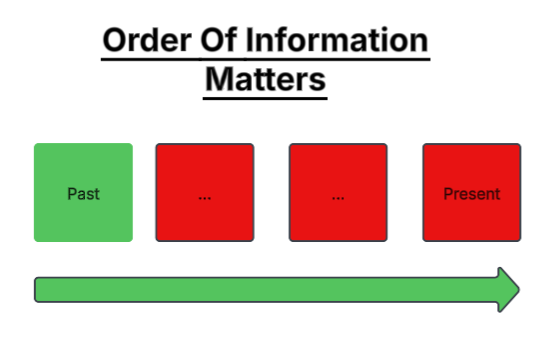
Figure 1: Is it always best for us to read all the historical data we have, describing a market?

An intelligent trader would rather begin with the most recent information and move backward, since older information quickly loses relevance in financial markets. This highlights a subtle truth unique to finance: information decays.

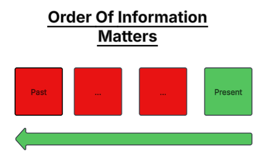
Figure 2: Or may we be better off by assuming that financial markets attribute more weight to the most recent information available?

In the natural sciences, information does not decay. Newton’s notes on gravity still yield the same results centuries later. But in financial markets, strategies that once worked in the 1950s may fail today. Market conditions evolve, and what was once valuable information often becomes “priced in” or obsolete.

This leads us to an important question: does using more historical data always improve predictive performance of our statistical models? Our findings suggest the opposite. Feeding a model too much data from the distant past can degrade its accuracy. As in the thought experiment we performed, one does not need to read every newspaper ever printed—only those still relevant to the present.

Professional human traders do not begin their analysis from the first recorded candle in every market they trade. Yet in machine learning, we expect our models to do so, blindly assuming that more is better. This discussion challenges that assumption and examines whether financial markets have an effective memory—a limit beyond which older information ceases to matter.

Our objective is to study the relationship between the amount of historical data used for training and our out-of-sample performance. We focus on whether a smaller, more recent subset of data can match or even outperform a model trained on the entire dataset. To investigate this, we used roughly eight years of market data and partitioned it in half. The training set grew into incremental segments—10%, 20%, 30%, and so on—adding progressively older data. One model was assigned to each partition.We then measured each model's error across a fixed test set of roughly 4 years.

The results were clear: the lowest out-of-sample error occurred from the model that was fit using only 80% of the available training data, not all of it. Adding older data beyond that point only worsened accuracy. This demonstrates that models can learn better with less data, especially if older observations no longer reflect current market realities.

The amount of data being used to train the model is intended to be a proxy for the costs associated with building the model. Generally speaking, the more data we use to train the model, the more expensive it becomes to obtain the model. Therefore, these findings carry important implications for practitioners at all levels. Understanding them helps reduce computational costs, cloud infrastructure costs, shorten development cycles, and improve model efficiency.

Getting Started With Our Analysis in Python

We will now begin analyzing the data exported from MetaTrader 5 using the standard Python libraries we typically rely on.

#Import the standard python libraries
import numpy as np
import pandas as pd
import seaborn as sns
import MetaTrader5 as mt5
import matplotlib.pyplot as plt

Now let us log in to the MetaTrader 5 terminal.

#Log in to our MT5 Terminal
if(mt5.initialize()):
   #User feedback
   print("Logged In")

else:
   print("Failed To Log In")

Logged In

Before we fetch historical data on a sybol, we must first select the symbol from the market watch.

#Fetch Data on the EURUSD Symbol
#First select the EURUSD symbol from the Market Watch
if(mt5.symbol_select("EURUSD")):
    #Found the symbol
    print("Found the EURUSD Symbol")

Found the EURUSD Symbol

Now we can fetch the quotes from our broker.

#Fetch the historical EURUSD data we need
data = pd.DataFrame(mt5.copy_rates_from_pos("EURUSD",mt5.TIMEFRAME_D1,0,3000))
data

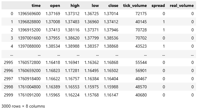
Figure 1: Getting started with our analysis of historical EURUSD market data.

The data by convention arrives to us in unix time, since most brokers implement linux servers. We will therefore, convert the time from seconds, to a human readable format of year-month-date.

#Convert the time from seconds to human readable
data['time'] = pd.to_datetime(data['time'],unit='s')
#Make sure the correct changes were made
data

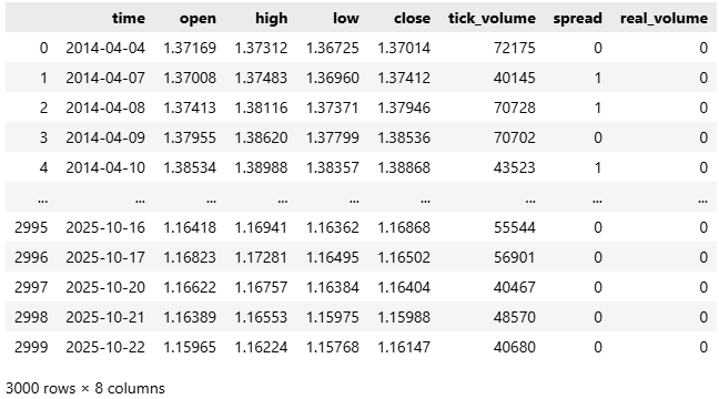
Figure 2: Converting our time denomination from seconds, to a human readable format.

Now let us focus, on the 4 columns that make the open, high, low and close price feeds.

#Select the OHLC columns
data = data.iloc[:,:-3]
data

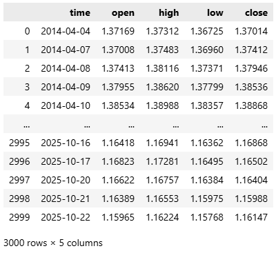
Figure 3: Reduce the dataset so we can focus our analysis on the four primary price levels.

Then, we start by building a classical time series forecasting model, where predictions are made one step into the future.

#Define the classical horizon
HORIZON = 1

Following this setup, we label our data.

#Label the data
data['Target'] = data['True Close'].shift(HORIZON)

Remove any missing rows, since missing values can cause errors when fitting models from scikit-learn.

#Drop missing rows
data.dropna(inplace=True)

Next, we import the necessary machine learning libraries.

#Import cross validation tools
from sklearn.linear_model import Ridge,LinearRegression
from sklearn.metrics import root_mean_squared_error
from sklearn.neural_network import MLPRegressor
    

Let us divide our dataset into two equal parts—one for training and one for testing.

#The big picture of what we want to test
train , test = data.iloc[:data.shape[0]//2,:] , data.iloc[data.shape[0]//2:,:]

We then separate the input features and output targets.

#Define inputs and target
X = data.columns[1:-1]
y = data.columns[-1]

To keep our workflow modular, we define a function called get_model(), which returns a Random Forest Regressor. Random Forests are powerful estimators capable of capturing complex, nonlinear interactions between variables that simpler models might miss.

#Fetch a new copy of the model
def get_model():
    return(RandomForestRegressor(random_state=0,n_jobs=-1))

With our model defined, we proceed to the main section of the program. Here, we create a list to record model performance scores and specify the total number of iterations we wish to run. Users are free to experiment with this parameter—larger iteration counts provide more detailed insights.

In each loop iteration, we train the model on an increasing fraction of the training data. Using NumPy’s arange function, we create fractions ranging from 0.1 to 1.0 in increments of 0.1. For each fraction, we train the model using only the most recent portion of the available training data and evaluate it on a fixed test set. This process repeats until the model has been trained on the entire training partition.

After all iterations are complete, we plot the model’s performance against the training fraction. The red marker on the graph highlights the lowest test error—observed at the 80% mark. This means the model achieved its best out-of-sample performance when trained on only 80% of the available data.

It is important to note that this procedure is not the same as classical k-fold cross-validation. In our setup, the training and test sets share no overlapping observations. The training set simply grows to include older data, while the test set remains fixed. Observing a performance minimum before reaching 100% suggests that the oldest data provided no additional predictive value.

In conclusion, our experiment demonstrates that a smaller, less expensive model—trained on a limited, more recent portion of data—can outperform a model trained on the entire historical dataset.

#Store our performance
error = []

#Define the total number of iterations we wish to perform
ITERATIONS = 10

#Let us perform the line search
for i in np.arange(ITERATIONS):
    #Training fraction 
    fraction =((i+1)/10)

    #Partition the data to select the most recent information
    partition_index = train.shape[0] - int(train.shape[0]*fraction)

    train_X_partition = train.loc[partition_index:,X]
    train_y_partition = train.loc[partition_index:,y]

    #Fit a model 
    model = get_model()

    #Fit the model
    model.fit(train_X_partition,train_y_partition)

    #Cross validate the model out of sample
    score = root_mean_squared_error(test.loc[:,y],model.predict(test.loc[:,X]))

    #Append the error levels
    error.append(score)

#Plot the results
plt.title('Improvements Made By Historical Data')
plt.plot(error,color='black')
plt.grid()
plt.ylabel('Out of Sample RMSE')
plt.xlabel('Progressivley Fitting On All Historical Data')
plt.scatter(np.argmin(error),np.min(error),color='red')

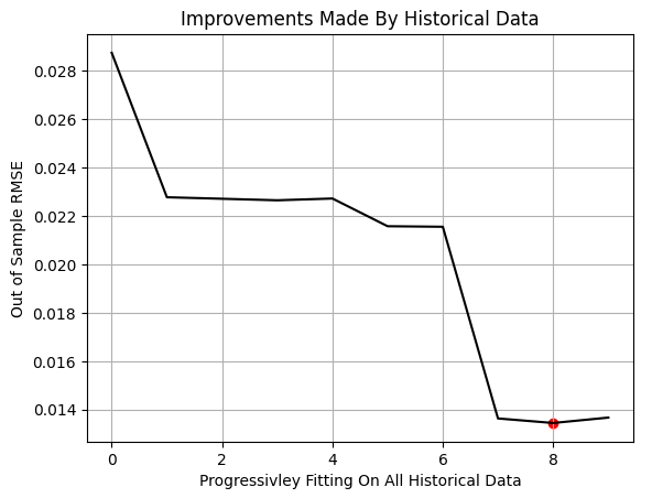
Figure 4: The results we obtained from our MetaTrader 5 terminal indicate that simply feeding more historical data does not always improve performance.

We now identify the optimal partition index estimated from our line search.

#Let us select the partition of interest
partition_index = train.shape[0] - int(train.shape[0]*(0.8))

Our methodology indicates that the first 300 observations—roughly one year of data—contained in the training set were not useful for prediction. 

train.loc[partition_index:,:]

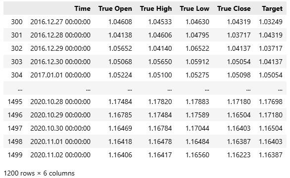
Figure 5: We have approximated the above subset of our training data to be most relevant to the present market.

Therefore, we will compare the performance of two models:

1. Classical model:trained on all available data and predicting one step ahead.
2. Modern variant: trained only on the optimal partition of all available historical data and designed to predict more than one step into the future.

Let us first establish a baseline performance level following the classical setup. To do this, we initialize a new model.

#Prepare the baseline model
model = LinearRegression()

Fit the model on the entire dataset, in line with the classical setup.

#Fit the baseline model on all the data
model.fit(train.loc[:,X],train.loc[:,y])

Next, we prepare to export the model to ONNX (Open Neural Network Exchange) format. ONNX provides a framework-independent way to represent and deploy machine learning models, allowing them to run on different platforms regardless of their training environment.

#Prepare to export to ONNX
import onnx
from skl2onnx import convert_sklearn
from skl2onnx.common.data_types import FloatTensorType

After loading the required dependencies, we define the input and output shapes of our model. 

#Define ONNX model input and output dimensions
initial_types = [("FLOAT INPUT",FloatTensorType([1,4]))]
final_types = [("FLOAT OUTPUT",FloatTensorType([1,1]))]

Convert the sklearn model to its ONNX prototype format using the convert_sklearn function. 

#Convert the model to its ONNX prototype
onnx_proto = convert_sklearn(model,initial_types=initial_types,target_opset=12)

Once converted, we save the ONNX model to disk with onnx.save().

#Save the ONNX model
onnx.save(onnx_proto,"EURUSD Baseline LR.onnx")

Getting Started in MQL5

At this stage, we are ready to establish our baseline performance benchmark. The first step is to define the system constants that will remain fixed throughout both tests, ensuring that any performance differences arise solely from our modeling choices.

//+------------------------------------------------------------------+
//|                                            Information Decay.mq5 |
//|                                               Gamuchirai Ndawana |
//|                    https://www.mql5.com/en/users/gamuchiraindawa |
//+------------------------------------------------------------------+
#property copyright "Gamuchirai Ndawana"
#property link      "https://www.mql5.com/en/users/gamuchiraindawa"
#property version   "1.00"

//+------------------------------------------------------------------+
//| System definitions                                               |
//+------------------------------------------------------------------+
#define SYMBOL "EURUSD"
#define SYSTEM_TIMEFRAME PERIOD_D1
#define SYSTEM_DATA COPY_RATES_OHLC
#define TOTAL_MODEL_INPUTS 4
#define TOTAL_MODEL_OUTPUTS 1
#define ATR_PERIOD 14
#define PADDING 2

Load the ONNX model. Recall that this baseline model was trained on all historical data and configured to predict one step ahead.

//+------------------------------------------------------------------+
//| System resources we need                                         |
//+------------------------------------------------------------------+
#resource "\\Files\\EURUSD Baseline LR.onnx" as const uchar onnx_buffer[];

Next, we load the necessary libraries—those for trade execution and our custom utility library, which retrieves essential trading information such as the minimum lot size and current bid and ask prices. 

//+------------------------------------------------------------------+
//| Libraries                                                        |
//+------------------------------------------------------------------+
#include <Trade\Trade.mqh>
#include <VolatilityDoctor\Trade\TradeInfo.mqh>
CTrade Trade;
TradeInfo *TradeHelper;

We also define a set of global variables to be used throughout the application.

//+------------------------------------------------------------------+
//| Global variables                                                 |
//+------------------------------------------------------------------+
long         onnx_model;
vectorf      onnx_inputs,onnx_output;
MqlDateTime current_time,time_stamp;
int         atr_handler;
double      atr[];

Once the setup is complete, we proceed with the initialization phase of the application. Here, we create the ONNX model instance from the buffer defined in the program’s header. We perform an error check by confirming that the model handle is valid. If an invalid handle is detected, an error message is displayed, and initialization is aborted. Otherwise, we proceed to define the model’s input and output shapes. Any errors encountered here are similarly reported to the user. If initialization succeeds, we then set the initial values of key global variables such as the current time, create new class instances, and initialize the technical indicator upon which our application depends.

//+------------------------------------------------------------------+
//| Expert initialization function                                   |
//+------------------------------------------------------------------+
int OnInit()
  {

//--- Create the ONNX model from its buffer
   onnx_model = OnnxCreateFromBuffer(onnx_buffer,ONNX_DATA_TYPE_FLOAT);

//--- Check for errors
   if(onnx_model == INVALID_HANDLE)
     {
      //--- User feedback
      Print("An error occured loading the ONNX model:\n",GetLastError());
      //--- Abort
      return(INIT_FAILED);
     }

//--- Setup the ONNX handler input shape
   else
     {
      //--- Define the I/O shapes
      ulong input_shape[] = {1,4};
      ulong output_shape[] = {1,1};

      //--- Attempt to set input shape
      if(!OnnxSetInputShape(onnx_model,0,input_shape))
        {
         //--- User feedback
         Print("Failed to specify the correct ONNX model input shape:\n",GetLastError());
         //--- Abort
         return(INIT_FAILED);
        }

      //--- Attempt to set output shape
      if(!OnnxSetOutputShape(onnx_model,0,output_shape))
        {
         //--- User feedback
         Print("Failed to specify the correct ONNX model output shape:\n",GetLastError());
         //--- Abort
         return(INIT_FAILED);
        }

      //--- Mark the current time
      TimeLocal(current_time);
      TimeLocal(time_stamp);

      //--- Setup the trade helper
      TradeHelper = new TradeInfo(SYMBOL,SYSTEM_TIMEFRAME);

      //--- Setup our technical indicators
      atr_handler = iATR(Symbol(),SYSTEM_TIMEFRAME,ATR_PERIOD);
      //--- Success
      return(INIT_SUCCEEDED);
     }
  }

When the application is no longer in use, we ensure proper resource cleanup by freeing memory allocated to the ONNX model, the technical indicator, and other dynamic objects created during runtime.

//+------------------------------------------------------------------+
//| Expert deinitialization function                                 |
//+------------------------------------------------------------------+
void OnDeinit(const int reason)
  {
//---
   OnnxRelease(onnx_model);
   IndicatorRelease(atr_handler);
   delete(TradeHelper);
  }

The main logic of the application resides in the OnTick() function. Each time a new market price arrives, we update the current time using the TimeLocal() function, which returns the local time of the computer running the MetaTrader 5 terminal. We then compare currenttime.dayofyear with timestamp.dayofyear.

Since Timestamp was last updated during initialization, this condition will only be passed once a full day has passed. When the condition fails, we update the timestamp to the current time, refresh the technical indicator buffers, and prepare the input and output vectors for the ONNX model.

We then request a new prediction from the model using the OnnxRun() command. This function takes the ONNX model instance, flag parameters for special model attributes, and the prepared input and output vectors.

After obtaining the prediction, we display feedback to the user. If no open trade conditions exist, we execute actions based on the model’s output. However, if the model fails to produce a prediction, we notify the user that an error has occurred.

//+------------------------------------------------------------------+
//| Expert tick function                                             |
//+------------------------------------------------------------------+
void OnTick()
  {
//--- Check for updated candles
   TimeLocal(current_time);

//--- Periodic one day test
   if(current_time.day_of_year != time_stamp.day_of_year)
     {
      //--- Update the time stamp
      TimeLocal(time_stamp);

      //--- Update technical indicators
      CopyBuffer(atr_handler,0,0,1,atr);

      //--- Prepare a prediction from our model
      onnx_inputs = vectorf::Zeros(TOTAL_MODEL_INPUTS);
      onnx_inputs[0] = (float) iOpen(Symbol(),SYSTEM_TIMEFRAME,0);
      onnx_inputs[1] = (float) iHigh(Symbol(),SYSTEM_TIMEFRAME,0);
      onnx_inputs[2] = (float) iLow(Symbol(),SYSTEM_TIMEFRAME,0);
      onnx_inputs[3] = (float) iClose(Symbol(),SYSTEM_TIMEFRAME,0);

      //--- Also prepare the outputs
      onnx_output = vectorf::Zeros(TOTAL_MODEL_OUTPUTS);

      //--- Fetch a prediction from our model
      if(OnnxRun(onnx_model,ONNX_DATA_TYPE_FLOAT,onnx_inputs,onnx_output))
        {
         //--- Give user feedback
         Comment("Trading Day: ",time_stamp.year," ",time_stamp.mon," ",time_stamp.day_of_week,"\nForecast: ",onnx_output[0]);

         //--- Check if we have an open position
         if(PositionsTotal() == 0)
           {
            //--- Long condition
            if(onnx_output[0] > iClose(SYMBOL,SYSTEM_TIMEFRAME,0))
               Trade.Buy(TradeHelper.MinVolume(),SYMBOL,TradeHelper.GetAsk(),TradeHelper.GetBid()-(atr[0]*PADDING),TradeHelper.GetBid()+(atr[0]*PADDING),"");

            //--- Short condition
            if(onnx_output[0] < iClose(SYMBOL,SYSTEM_TIMEFRAME,0))
               Trade.Sell(TradeHelper.MinVolume(),SYMBOL,TradeHelper.GetBid(),TradeHelper.GetAsk()+(atr[0]*PADDING),TradeHelper.GetAsk()-(atr[0]*PADDING),"");
           }

         //--- Manage our open position
         else
           {
               //--- This control branch remains empty for now
           }
        }

      //--- Something went wrong
      else
        {
         Comment("Failed to obtain a prediction from our model. ",GetLastError());
        }
     }
  }
//+------------------------------------------------------------------+

Lastly, undefine all the system constants we created earlier. 

//+------------------------------------------------------------------+
//| Undefine system constants                                        |
//+------------------------------------------------------------------+
#undef SYMBOL
#undef SYSTEM_DATA
#undef SYSTEM_TIMEFRAME
#undef ATR_PERIOD
#undef PADDING
#undef TOTAL_MODEL_INPUTS
#undef TOTAL_MODEL_OUTPUTS

With our application defined, we are now ready to begin testing. We conduct our evaluation over the five-year backtest window previously identified. We start by selecting the baseline version of the application that we have just built and defining the corresponding training dates.

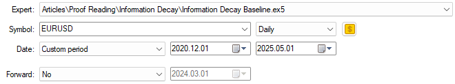
Figure 6: The dates we selected for our backtest period are outside the training period we identified in Figure 3.

Next, we specify the emulation conditions under which the backtest will run. Recall that we use every tick based on real ticks to capture a realistic evolution of market conditions. The delay setting is configured to random delay; this renders us a reliable emulation of the unpredictable nature of live trading environments.

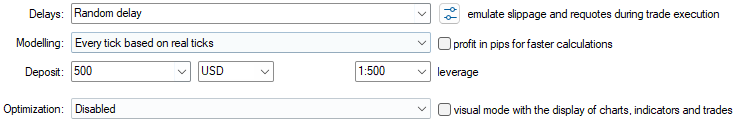
Figure 7: The backtest conditions we have selected are intended to emulate the chaos of real market conditions.

When reviewing the baseline performance, we observe that the initial version of our application produced a total profit of $90 over the five-year backtest period. While this outcome is not entirely poor, it is far from impressive. A closer look reveals an alarming characteristic in the trade composition: the application executed no long trades whatsoever throughout the entire backtest. All trades placed were exclusively short positions. This behavior was neither expected nor intended during development, and no clear explanation exists for why the model behaved this way. Additionally, the strategy accuracy was approximately 50%, barely above chance. Even more concerning, the expected payoff was negative, indicating that the application would likely lose money over the long run. 

Figure 8: A detailed statistical analysis of the results we have obtained from the back test we performed.

When examining the equity curve, we can see pronounced volatility and instability throughout the testing period. As we approach November 2022, the account balance stops growing and enters a prolonged consolidation phase that persists for nearly three years within the backtest window. Overall, the baseline model fails to grow the account meaningfully and provides little confidence in its long-term viability.

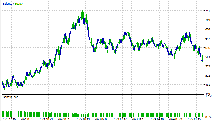
Figure 9: Visualizing the equity curve we obtained from following the traditional guidelines on how to build a statistical model.

Modifying Our ONNX Model

Now that we have established this baseline performance—obtained under the classical setup—let us move beyond the traditional framework and modify our ONNX model to better reflect how professional human traders actually operate. The first major modification departs from the conventional design philosophy. Instead of developing models that look only one step ahead, we now design our model to anticipate ten steps into the future. Human traders do not trade candle by candle; they act based on a broader picture of anticipated market movement. Our model should therefore reflect that same forward-looking intuition.

HORIZON = 10

Next, we identify the optimal data partition estimated using cross-validation techniques. 

#Let us select the partition of interest
partition_index = train.shape[0] - int(train.shape[0]*(0.8))
train.loc[partition_index:,:]

We then load a fresh model—identical in architecture to the baseline model. 

#Prepare the improved baseline model
model = LinearRegression()

Train the new model exclusively on this optimal partition of the data.

#Fit the improved baseline model
model.fit(train.loc[partition_index:,X],train.loc[partition_index:,y])

Once trained, we convert this improved model into its ONNX prototype. But recall that both models are of the same complexity.

#Convert the model to its ONNX prototype
onnx_proto = convert_sklearn(model,initial_types=initial_types,target_opset=12)

Finally, save the ONNX model to a file.

#Save the ONNX model
onnx.save(onnx_proto,"EURUSD Improved Baseline LR.onnx")

Improving Our Initial Results

The user should note that the only component requiring modification is the ONNX file resource reference located in the application’s header. The rest of the system remains unchanged and will operate exactly as before.

//+------------------------------------------------------------------+
//| System resources we need                                         |
//+------------------------------------------------------------------+
#resource "\\Files\\EURUSD Improved Baseline LR.onnx" as const uchar onnx_buffer[];

We then select this improved version of the application to be tested over the same five-year window as the baseline model. Importantly, all backtest conditions—including random delay and tick-based execution—are kept identical to those used in Figure 7 to ensure comparability.

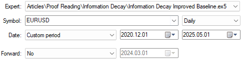
Figure 10: Selecting our new and improved version of the application to compare the improvements we have realized.

When analyzing the detailed performance statistics, the difference between the two applications becomes immediately apparent. The total net profit of the improved model has increased by more than threefold, rising from roughly $90 to $330. We can now observe that the initial skew in the distribution of trades has been fully corrected. In the baseline version of our application, all trades were exclusively short positions—an unintended imbalance in the model’s behavior. In contrast, the improved version now places both long and short trades in a balanced manner, reflecting the more natural decision-making process of a real human trader.

Additionally, there is a remarkable improvement in accuracy, rising from approximately 52% to nearly 60%. This is an encouraging development, suggesting that the model’s internal decision logic has become more consistent and discerning.

However, what I found most surprising in this analysis is that the total number of trades remained identical between both models. Each version executed exactly 152 trades during the backtest. Despite this, the improved model achieved more than triple the total net profit, demonstrating a clear increase in efficiency. In other words, with the same number of trades, the improved model generated substantially higher returns. Moreover, both the Sharpe ratio and the expected payoff have risen significantly — further evidence that the model is allocating its capital and timing its trades more intelligently.

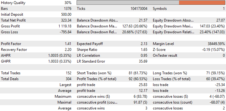
Figure 11: A detailed analysis of the results we have obtained indicates that the changes we have made were appropriate.

When examining the equity curve produced by the improved version, the difference is striking. The prolonged consolidation period that plagued the initial application—which lasted nearly three years—has completely disappeared. The new model shows steady and consistent growth, indicating that whatever structural limitations or blind spots existed in the earlier version have now been effectively resolved. This outcome is both encouraging and validating, confirming that the refinements we introduced had a meaningful impact.

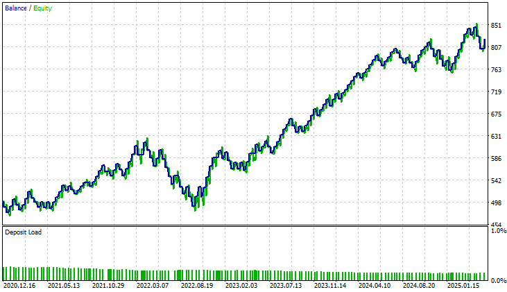
Figure 12: The improved equity curve we have produced demonstrates that the changes we made brought stability into our system over a 5 year test.

Conclusion

After reading this article, the reader should walk away empowered with actionable insights into the true nature of statistical learning in algorithmic trading. One key takeaway is that blind adherence to traditional statistical principles does not necessarily serve us as algorithmic traders. We cannot simply borrow the heuristics of “big data” and expect them to work unchanged in our domain — where the relevance of data is heavily weighted toward the present.

This article has also provided practical guidance for conserving capital that might otherwise be misused in acquiring overly complex or inefficient models. The insights presented here can translate directly into real financial savings, not only in capital expenditure but also in compute resources, development time, and infrastructure costs associated with deploying advanced machine learning systems.

Finally, the reader should now have a clearer focus on the blind spots inherent in classical cross-validation paradigms. We often overlook whether all the data we include truly contributes toward achieving our objective. The analysis presented here exposes a new form of overfitting—one that classical statistical learning provides little guidance on. It shows that attempting to train a model on all available data can itself be an unrecognized source of inefficiency. Taken together, these lessons equip us to build more effective, efficient, and profitable machine learning models for algorithmic trading.

File Name	File Description
Information Decay Baseline.mq5	The baseline trading application built using classical machine learning paradigms.
Information Decay Improved Baseline.mq5	The improved application developed using Effective Memory Cross-Validation (EMCV) — a domain-bound technique introduced in this work.
Limitations of Cross Validation 1.ipynb	The Jupyter Notebook used to analyze market data and build our ONNX models.
EURUSD Baseline LR.onnx	The classical ONNX model built following classical best practices .
EURUSD Improved Baseline LR.onnx	The enhanced ONNX model that outperformed the classical benchmark by following new domain-bound best practices discussed here.