Seasonality Filtering and time period for Deep Learning ONNX models with python for EA

Introduction

When I read the article: Benefiting from Forex market seasonality, I thought of this to make this what I think is an interesting article. I could start comparing an EA with and without seasonality's and with to see if it can benefit. 

I all ready new that markets depend on seasonality since I read that the Mark Zuckerberg got the money for Facebook, from an investor that got his money investing the one that they gave him in the Bar Mitzvah in stocks of petrol when the climate in the Caribbean  there were going to have hurricanes. He first studied the climate and forecasted that there would be a bad weather during a period of time.

I'm very proud and interested in writing this article, since if the results are not better, even though I know that market and seasonality are good companions. I good approach to making this  come true, would be to merge both EA's in one, but we already have an article about that, here's the link:  An example on how to ensemble ONNX models in mql5.

First of all we will compare models with and without filtering with using an EA, to see how filtering data affects or not, and, after this, we will discuss seasoning with a graph, to end up with a real case of study, for February 2024, with and without seasoning. In the last part of the article (which I find very interesting), we will discuss other approaches to the EA we already have from the article: How to use ONNX models in MQL5 , and we will see if we can benffit of finetuning those EA's and ONNX models, and yes, the answer is that yes we can.)

To make this happen, we will first download the data (all ticks) with this script: Download all data from a symbol (please support this article buying this script). We just have to add the script to the symbol chart we need to study, and, in some time (less than an hour) we will have downloaded all the historic ticks from that symbol in our Files folder.

When we have all the ticks downloaded, we will work with that csv, and extract only the data we need or want (in this case, the periods from January to February 2015 to 2023).

Seasonality

Seasonality in trading is all about spotting the regular ebbs and flows in asset prices that happen predictably throughout the year. It's like recognizing that certain stocks tend to do better at certain times than others. Let's unpack this idea a bit.

Understanding Seasonality in Trading:

• Definition: Seasonality means noticing how prices tend to fluctuate in a recurring pattern based on the time of year. This could be tied to actual seasons (like summer or winter), commercial seasons (such as the holiday rush), or even specific months.
• Examples: Smart investors keep an eye on these patterns because they're often reliable and profitable. Here are a few examples:
  • Weather-Related Seasonality: Just like the weather affects farming seasons, it also impacts things like commodity prices and related stocks. For instance, a company selling beach gear might see a boost in sales during summer but a dip in colder months, affecting its stock.
  • Holiday Seasonality: Retail stocks often see a bump during holiday shopping frenzies. Companies that thrive on holiday sales, like gift shops, tend to shine during these times.
  • Quarterly Earnings Seasonality: Publicly traded companies report earnings every quarter, and their stock prices can react predictably during these seasons.
  • Tax Seasonality: Tax-related events can shake up the market, especially for sectors tied to finance.
  • Natural Cycles: Industries like tourism or energy have their own seasonal demand patterns, like summer vacations or winter heating needs.

Trading Strategies Based on Seasonality:

• Traders can leverage seasonality in a few ways:
  • Identifying Seasonal Patterns: Digging into past data to spot trends that repeat at certain times of the year.
  • Timing Trades: Making moves in and out of positions based on these seasonal trends.
  • Managing Risk: Adjusting how much risk you're taking on during volatile periods.
  • Sector Rotation: Switching up investments between sectors that tend to perform better at different times of the year.

Filtering Data

We will use the Low-pass filter. According to Wikipedia:

A low-pass filter is a filter that passes signals with a frequency lower than a selected cutoff frequency and attenuates signals with frequencies higher than the cutoff frequency. The exact frequency response of the filter depends on the filter design. The filter is sometimes called a high-cut filter, or treble-cut filter in audio applications. A low-pass filter is the complement of a high-pass filter.

Why do we choose low-pass filters over high-pass filters in algorithmic trading? In algorithmic trading, the preference for low-pass filters stems from several key advantages:

1. Signal Smoothing: Low-pass filters effectively smooth out noisy price movements, emphasizing longer-term trends over short-term fluctuations.
2. Reducing High-Frequency Noise: They help attenuate high-frequency noise, which may not provide meaningful information for trading strategies.
3. Lower Transaction Costs: By focusing on longer-term trends, low-pass filters can lead to fewer, more strategic trades, potentially reducing transaction expenses.
4. Better Risk Management: Low-pass filters contribute to a more stable and predictable trading strategy, reducing the impact of short-term market fluctuations.
5. Alignment with Investment Horizon: They are well-suited for strategies with longer-term investment horizons, capturing trends over extended periods effectively.

I personally use low-pass filter to filter high frequencies. It does not have much sense to use a high-pass filter here.

This is what we will use (note: I ended up changing the order and cutoff_frequency parameters in the last part of the article to 0.1 cutoff and order equal to 1, because they ended up giving better results. Also, the correct .py to filtering are the ones of the last part of the article (there I used not only better parameters, I also used minmaxscaler to fit and inverse. so the ones to use, are those)).

# Low-pass filter parameters
cutoff_frequency = 0.01  # Cutoff frequency as a proportion of the Nyquist frequency
order = 4

# Apply the low-pass filter
def butter_lowpass_filter(data, cutoff, fs, order):
    nyquist = 0.5 * fs
    normal_cutoff = cutoff / nyquist
    b, a = butter(order, normal_cutoff, btype='low', analog=False)
    print("Filter coefficients - b:", b)
    print("Filter coefficients - a:", a)
    y = lfilter(b, a, data)
    return y

filtered_data_low = butter_lowpass_filter(df2['close'], cutoff_frequency, fs=1, order=order)

We will make use of "onnx_LSTM_simple_filtered.py" and  "onnx_LSTM_simple_not_filtered.py" to make the ONNX models and compare them.

Note: I've used a model v1 and a model v2 that have different Low-pass filter parameters.

This are the results:

We will use the same inputs for the EA's

The time period to study, will be from the first of February to the first of March.

For the not filtered model:

RMSE         : 0.0010798043714784716
MSE          : 1.165977480664017e-06
R2 score     : 0.8799146678247277

Filtered v1

# Parámetros del filtro pasa bajo

cutoff_frequency = 0.01  # Frecuencia de corte en proporción a la frecuencia de Nyquist

order = 4

RMSE         : 0.0010228999869332884
MSE          : 1.0463243832681218e-06
R2 score     : 0.8922378749062259

Filtered v2

cutoff_frequency = 0.1  # Frecuencia de corte en proporción a la frecuencia de Nyquist

order = 2

RMSE         : 0.0010899163515744447
MSE          : 1.1879176534293484e-06
R2 score     : 0.8775550550819025

Conclusion over filtering

It yields better results only when using the correct parameters.

So, yes. Its convenient to use filtering.

Code used and models:

ONNX.eurusd.H1.120.Prediction_FILTERED.mq5

ONNX.eurusd.H1.120.Prediction_FILTERED_v2.mq5 ONNX.eurusd.H1.120.Prediction_NOT_FILTERED.mq5

onnx_LSTM_simple_EURUSD_filtered.py

onnx_LSTM_simple_EURUSD_not_filtered.py

Download all data from a symbol EURUSD_LSTM_120_1h_not_filtered.onnx EURUSD_LSTM_120_1h_filtered_v1.onnx EURUSD_LSTM_120_1h_filtered_v2.onnx

Are symbols seasonal?

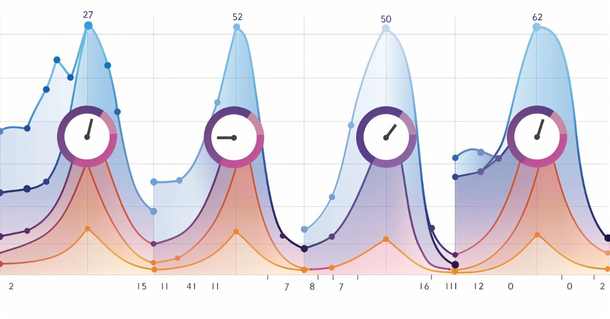
For this part, we will first see this in a graph, we will get the data from February since 2015 to 2023 and we will add the data to see how it moves arround those weeks.

This is what we can see from that period:

Conclusion:

We can see it has some tendencies, or at least we don't se a black (sum line) horizontal line. There are gaps between each line, because the symbol trades over the year and it prices fluctuate. This is why in the next part of the article, we will concatenate all the symbols by years for February and this is why we need to use a filter, so it doesn't pass the high frequency from the for example last date of 2022 to the first of February 2023 and when the AI gets trained of for example the close of a Friday and the open of a Monday, so, it doesn't study those changes and seeks a more smoothened data.

scripts and data used:

Download all data from a symbol Download_seasonalities_1h_v2.py data febs.zip draw_with_sum.py

Is this data from the symbol correlated?

The autocorrelation is a characteristic of the data that shows the degree of similarity between values in successive time intervals.

A value near 1 indicates that there is a big positive correlation.

This are the results we obtained with the  autocorrelation.py

[1.         0.99736147 0.99472432 0.99206626 0.98937664 0.98671649
 0.98405706 0.98144222 0.9787753  0.97615525 0.97356318 0.97099777
 0.96848029 0.96602671 0.96360361 0.96113539 0.95865344 0.95615626
 0.95362417 0.95108177 0.94854957 0.94599045 0.94346076 0.94091564
 0.93837742 0.93583734 0.9332909  0.93074655 0.92826504 0.92579028
 0.92330505 0.92084645 0.91834403 0.91581296 0.91328091 0.91076099
 0.90826447]

Creating a ONNX model for February seasons

For this task, we just have to concatenate all data into one single csv, and, make a model with it.

we will use the create concat seasonal .py to make one single csv, that is added to the zip seasonal_feb_contac. With the onnx_LSTM_..._seasonals.py we will train and create the model.

Scripts and data used:

seasonal_feb_concat.zip create_concat_seasonal_data.py

onnx_LSTM_simple_EURUSD_concat_seasonals.py

Testing results for the seasonal model and comparing it to the 120 days (1h) filtered model

Seasonal model

RMSE         : 0.013137568368684325
MSE          : 0.00017259570264185493
R2 score     : 0.7166764010650979

This are not astonishing results, but, the results look overall good (it doesn't have many negative Sharpe results)

If we compare it to the filtered model,

What I've found curious, is that the number of negative Sharpe values occupies half of the table from the optimization for the filtered model, while the negative ones for the seasonal model occupies around a fifth of the table. This is notable, because even having a lower r2, it seems to be a robust model giving profitable returns.

I could have also tested the EA without SL and TP, but a find a better practice to always use them in EA's.

Code and ONNX model used:

ONNX.eurusd.H1.120.Prediction_seasonal.mq5 EURUSD_LSTM_270_1h_filtered_seasonal0.72.onnx onnx_LSTM_simple_EURUSD_concat_seasonals.py

What time period use?

For this part of the article, I've finetuned the filter to have better results for EURUSD

cutoff_frequency = 0.1  # Frecuencia de corte en proporción a la frecuencia de Nyquist
order = 1

I also modified the filter:

from sklearn.preprocessing import MinMaxScaler
from scipy.signal import butter, lfilter

# Parámetros del filtro pasa bajo
cutoff_frequency = 0.1  # Frecuencia de corte en proporción a la frecuencia de Nyquist
order = 1

# Aplicar filtro pasa bajo
def butter_lowpass_filter(data, cutoff, fs, order):
    nyquist = 0.5 * fs
    normal_cutoff = cutoff / nyquist
    b, a = butter(order, normal_cutoff, btype='low', analog=False)
    print("Coeficientes del filtro - b:", b)
    print("Coeficientes del filtro - a:", a)
    y = lfilter(b, a, data)
    return y

scaled = MinMaxScaler(feature_range=(0,1))

valores_df1 = df.filter(['close']).values
valores_df1 = pd.DataFrame(valores_df1)
x_features1 = valores_df1[[0]]
valores_df2 = x_features1.values


data_escalada = scaled.fit_transform(valores_df2)

print(data_escalada)

filtered_data_low = butter_lowpass_filter(data_escalada, cutoff_frequency, fs=1, order=order)
print("filtered_data_low",filtered_data_low)

filtered_data_low_unscaled = scaled.inverse_transform(filtered_data_low)

The order, must be an order around the price as an integer.

This strategy tests, are done over a month period for the 1 h strat, on February 2024. For the 30 min strat, its used from first of February to the 15th of February and so on ...

For 15 min I've done tests with and without filters, and the results conclude that doing a filter with its finetune, give better results (at least overall).

15 min with filter (Sharpe)

LTSM_simple_15m_filtrado.py LSTM.15m.EURUSD.120.0.98.onnx ONNX.eurusd.H1.120.15m_eurusd.mq5

15 min without filter

LTSM_simple_15m_filtrado_sin.py LSTM.15m.EURUSD.120.0.98.onnx ONNX.eurusd.H1.120.15m_eurusd.mq5

30 min with filter (now on I will always use filter)

LSTM.30m.EURUSD.120.0.94.onnx LTSM_simple_30m_filtrado.py ONNX.eurusd.H1.120.30m_eurusd.mq5

1 hour

1 hour files.zip (815.64 KB)

2 hours

As I can't use a two day period, I used one day period (for the next days value in the EA)

2h.zip

As I can't load more than 32 files, the next files will all be uploaded in a folder.

Conclusion

It seems that with this strat, as the period goes higher, the results look more robust for all the TP's and SL's

NextDay var

I've used the strategy from this article : How to use ONNX models in mql5, but as I've had good results with the 2hours strat, and in that one I used 1Day period. We will study other values for the NextDays var

   if(TimeCurrent()>=ExtNextDay)
     {
      GetMinMax();
      //--- set next day time
      ExtNextDay=TimeCurrent();
      ExtNextDay-=ExtNextDay%PeriodSeconds(PERIOD_D1);
      ExtNextDay+=PeriodSeconds(PERIOD_D1);
     }

void GetMinMax(void)
  {
   vectorf close;
   close.CopyRates(_Symbol,PERIOD_D1,COPY_RATES_CLOSE,0,SAMPLE_SIZE);
   ExtMin=close.Min();
   ExtMax=close.Max();
  }

We will now proceed to study EURUSD with period 30min with filtered data, and different NextDay periods (We will use 1D, 12h and 6h) and discuss results.

1D with 30 min period

12 H  with 30 min period

6h 30 min period

The results seem better when finetuning the NextDay var. Lets see how it evolves in lower NextDay periods.

30 min with NextDay periods of 4h

30 min with NextDay periods of 2h

30 min with NextDay periods of 1h

It seems that for at least 30 minute periods, around 8 to 12 bars of 30 minutes give better results.

As this "game" is to win more money, and one way to do that is to have more winning trades and a solid strategy. Lets see if we can use this start to win with 5 minutes periods, so we will try this strat for 5 minutes and 1 h and 30 min for the NextDay var.

5 minutes with 1 h NextDay var.

5 minutes with 30 min NextDay var.

Files used:   Last files.zip

Other time periods, seem to be more reliable, but, if you want another EA, you have more to use.

For last, we can make adjustments to the strategy, that could end up giving better results or more solid results, like establishing a limit of time or bars, for example, in 1 h periods, and using a 12h for next day, we could establish that once the order is made, it must stay opened no more than 12 hours.

   if(ExtPredictedClass>=0)
     {
      if(PositionSelect(_Symbol))
         CheckForClose();
      else
        {
         CheckForOpen();
         started_time1 = rates[0].time;
         string started_time1_str = TimeToString(started_time1);

int total = PositionsTotal();
   if(total>0)
     {
      datetime started_time2 = rates[0].time;
      string started_time2_str = TimeToString(started_time2);
      int segundos = started_time2 - started_time1;
      Print("Tiempo 1: ", started_time1_str);
      Print("Tiempo 2: ", started_time2_str);
      Print("Diferencia en segundos: ", segundos);
      if((segundos >= days*PeriodSeconds(PERIOD_H12)) && segundos != 0)
        {
         Print("closing position----------------");
         ExtTrade.PositionClose(_Symbol,3);

        }
     }

ONNX.eurusd.120.1h_H12_eurusd.v3.mq5 (9.23 KB)

Conclusion

We have seen seasoning, filtering and compared models, EA's an parameters for the EA's to get better results with finetuning. I hope you enjoyed reading this article as I enjoyed making it.