Modified Grid-Hedge EA in MQL5 (Part III): Optimizing Simple Hedge Strategy (I)

Introduction

Welcome to the third installment of our "Optimizing a Simple Hedging Strategy" series. In this segment, we'll begin with a brief review of our progress to date. So far, we have developed two key components: the Simple Hedge Expert Advisor (EA) and the Simple Grid EA. This article will focus on further refining the Simple Hedge EA. Our goal is to improve its performance through a combination of mathematical analysis and a brute force approach to find the most effective way to implement this trading strategy.

This discussion will focus primarily on the mathematical optimization of the Simple Hedge strategy. Due to the complexity and depth of the analysis required, it is impractical to cover both the mathematical optimization and the subsequent code-based optimization in a single article. Therefore, we'll devote this article to the mathematical aspects, ensuring a thorough exploration of the theory and calculations behind the optimization process. In subsequent articles of the series, we will shift our focus to the coding aspect of optimization, applying practical programming techniques to our theoretical foundations established here.

Here's what we plan to cover in this article:

1. Diving Deep into Optimization: A Closer Look
2. Mathematical Optimization
3. Conclusion

Diving Deep into Optimization: A Closer Look

When we say the word "optimization," what comes to mind? It's a term that's as broad as it is complicated, and it often raises the question: "What exactly is optimization?"

Let's break it down. At its core, optimization refers to the act, process, or methodology of refining something-be it a design, a system, or a decision-to its highest level of perfection, functionality, or effectiveness. But let's face it, achieving absolute perfection is more of an idealistic pursuit. The real goal? To push the boundaries of what's possible with the resources we have, and to strive for the best possible outcome.

As we delve deeper, it's clear that the realm of optimization is vast, with myriad methods at our disposal. In the context of this discussion, our focus will be on the "classic hedging strategy". Among the plethora of optimization techniques, two standout approaches will be the cornerstone of our exploration:

1. Mathematical Optimization: This approach uses the sheer power of mathematics to our advantage. Imagine being able to create profit functions, drawdown functions, and more, and then use these constructs to fine-tune our strategy based on solid, quantifiable data. It's a method that not only increases the precision of our optimization efforts, but also provides a clear, mathematical path to improving the effectiveness of our strategy.

2. Brute-Force Approach: At the other end of the spectrum is the brute-force approach, which is simple but daunting in its scope. This method involves testing every conceivable combination of inputs, backtesting each one to find the best possible configuration. The goal? To either maximize profits or minimize drawdowns, depending on our strategic priorities. But it's important to acknowledge the elephant in the room: the overwhelming number of input combinations. This complexity makes backtesting every possible scenario a Herculean task, especially with limited resources and time.
   

This is where the beauty of combining the two approaches comes in. By applying mathematical optimization first, we can significantly reduce the number of cases to brute force. It's a strategic maneuver that allows us to focus on the most promising configurations, making the brute-force process much more manageable and time-efficient.

In essence, the journey through optimization is a balancing act between theoretical precision and practical feasibility. Starting with mathematical optimization sets the stage by filtering through the vast sea of possibilities. Then, moving to brute force allows us to rigorously test and refine the remaining options. Together, these methods form a powerful duo that guides us toward the most effective optimization of our classic hedging strategy.

Mathematical Optimization

When venturing into the world of mathematical optimization, the first step is to establish a clear and actionable framework. This means delineating the variables that have a significant impact on our outcome-in this case, profit. Let's dissect the components that play a critical role in shaping our profit function:

1. Initial Position (IP): A binary variable, where 1 signifies a buy action and 0 indicates a sell action. This initial choice sets the stage for the trading strategy's direction.
2. Initial Lot Size (IL): The magnitude of the first order within a trading cycle, laying the groundwork for the scale of transactions.
3. Buy Take Profit (BTP): The predetermined profit threshold for buy orders, serving as a target for when to close positions and secure gains.
4. Sell Take Profit (STP): Analogously, this is the profit target for sell orders, marking the point at which sell positions are closed to realize profits.
5. Buy-Sell Distance (D): The spatial parameter defining the interval between buy and sell order levels, influencing the entry points for trades.
6. Lot Size Multiplier (M): This factor escalates the lot size for subsequent orders, introducing a dynamic adjustment based on the trading cycle's progression.
7. Number of Orders (N): The total count of orders within a cycle, encapsulating the breadth of the trading strategy.

For the sake of clarity, these parameters are presented in their simplified forms, although it's worth noting that in equations, some of these variables would be referred to with subscript notation.

With these parameters as our foundation, we can now proceed to formulate our profit function. The essence of this function is to mathematically represent how our profit (or loss) is affected by varying these variables. The profit function is a cornerstone of our optimization process, allowing us to quantitatively analyze the results of different trading strategies under different scenarios.

Now let us write the parameters of our profit function:

So our final profit function will look like this:

At first glance, the Profit function may seem daunting with its mathematical expressions and symbols. However, there's no need to be intimidated. Each component of the equation has a specific role and, when broken down, contributes to a comprehensive understanding of how profits are generated within our trading framework.

Now it is important to understand the dynamics of profit calculations. Central to this understanding is the distinction between the main profit function, denoted p(x), and its component, g(x), where x represents the total number of orders or positions. This distinction is crucial because it lays the foundation for understanding how profits are generated when a trading cycle is completed over x positions. Let's methodically deconstruct this concept to fully grasp its essence.

Suppose we decide to close the trading cycle with a single order. The scenario unfolds as follows:

In this setup, g(x) takes the value based on the interaction between the number of orders (N) and the initial position (IP). For example, if we set the Initial Lot Size (IL) to 0.01 and, for the sake of this explanation, let N be 1 and let the Initial Position (IP) denote a Buy action (i.e. IP = 1), then g(x) will take the value of Buy Take Profit (BTP). As a result, our profit function p(x) becomes 100 times 0.01 times BTP = BTP, symbolically indicating that our profit is equal to BTP. This illustration highlights an important point: we are calculating profits in pips, not in currency. This approach is deliberately chosen to generalize the profit calculation across different currencies, to ensure applicability regardless of account type (micro or standard) and to simplify the overall calculation. The rationale behind multiplying the lot size by 100 is simple - it facilitates the conversion of the lot size into an accurate pip value, an essential step for accurate profit calculation.

Now let's consider the scenario where N is increased to 2, introducing a new layer of complexity:

This slight adjustment complicates our profit calculation and invites a deeper exploration of the underlying reasons, which are best illustrated through examples. A critical component of this complexity is the introduction of the "floor" function, a mathematical operation reminiscent of what we learn in school as the Greatest Integer Function (GIF). The floor function serves a specific purpose: given any numeric value, it truncates the decimal component to the greatest preceding integer. For positive values, this operation is straightforward: floor(1.54) = 1, floor(4.52) = 4, and so on. This mechanism is integral to our profit function and ensures that only integer values are considered in the calculations, a simplification that keeps our focus on positive values and avoids the need to consider negative values in this context.

The initial segment of our formula begins by calculating the floor as -100 times the Impact Level (IL), illustrated by the case where IL equals 0.01. This results in a calculation of -100 times 0.01, which equals -1. When we integrate this with the Distance (D), the equation represents the loss of D pips for each trade that does not result in a profit, as outlined in the trading strategy. The next step is to add the floor of 100 times IL times the multiplier (M) to a function, g(x), which represents the Take Profit (TP) value, either for a buy or sell order. The product of IL and M determines the lot size for the subsequent (second) order, and multiplying this product by 100 facilitates the accurate calculation of pips.

A key question arises regarding the need for the floor function in our equation. To clarify, consider an example where IL is 0.01 and M is 2, resulting in a calculation of 100 times IL times M, which equals 2. In this case, applying the floor function to 2 yields 2, which seems to make the floor function redundant. However, the usefulness of the floor function becomes apparent in a different scenario: if IL remains at 0.01 and M is set to 1.5, the product of 100 times IL times M equals 1.5. At this point, it's important to realize that the resulting lot size of 0.015 is not allowed because brokers require lot sizes in multiples of 0.01. According to the strategy, the order size would revert to 0.01, with subsequent lot sizes increasing in a controlled manner to ensure that they remain viable under the broker's restrictions. For example, the next lot size calculated as 0.01 times 1.5 times 1.5 equals 0.0225, which effectively rounds to 0.02 for practical purposes. Therefore, the floor function is used to adjust the equation to this operational reality, ensuring that lot sizes such as 0.01 and subsequently 0.02 are accurately represented. This adjustment ensures that the model reflects the pragmatic constraints of trading and emphasizes the need for the floor function to accommodate the fractional increase in lot sizes under the strategy's guidelines. Finally, this adjusted value is multiplied by g(x), which corresponds to either the Buy TP or the Sell TP, further integrating the trading strategy parameters into the equation formulation. This detailed breakdown clarifies the rationale behind each component of the equation and emphasizes the strategic considerations inherent in its construction.

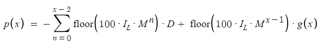
Now suppose N is 3, then we get a profit:

In the scenario where N is set to 3, the formula illustrates a situation where a profit is made under certain conditions, resulting in a structured approach to calculating results based on the number of orders denoted by N. The first segment remains consistent and represents a loss on the first order. The second segment adapts this approach by replacing g(x) with D, also reflecting a second order loss. The distinction in the third segment comes with the introduction of M^2, which indicates an exponential increase in the multiplier effect, which is straightforward given the context.

Extending this framework for different values of N, a generalized equation is presented that comprehensively encapsulates the dynamics of this trading strategy. This equation, adaptable to different instances of N, serves as a basic model for understanding the progression and potential outcomes as the number of orders increases.

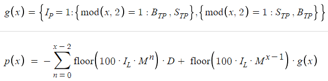
The determination of g(x), which alternates between Buy Take Profit (BTP) and Sell Take Profit (STP), depends on the Initial Position (IP) and the parity of N. This binary decision process is elegantly summarized in a conditional structure where the outcome is influenced by both the IP and the numerical characteristic of N, with emphasis on its evenness or oddness. This mechanism ensures a logical assignment of g(x) values that aligns with strategic objectives based on market position and order sequence.

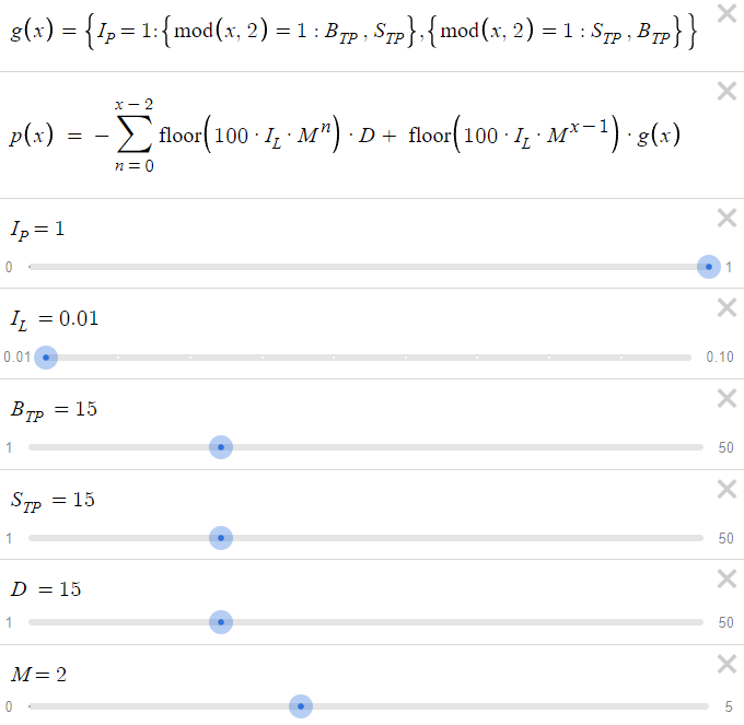
The use of Desmos, a graphing tool, facilitates interactive exploration of this equation by allowing parameter adjustments in real time, enhancing understanding through immediate feedback on changes. This tool's ability to display integer-specific results is particularly valuable in the practical context where the number of orders is an inherently discrete variable.

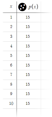
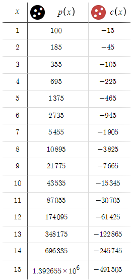
Desmos' demonstration with predefined parameters shows the model's behavior under standard conditions and reveals that a consistent profit of 15 pips can be expected over a spectrum of up to 10 orders.

Observing the results may create a desire to invest in this strategy; however, it is essential to exercise caution and not rush into any decisions. There are still numerous challenges and issues that need to be addressed before proceeding. To gain a more comprehensive understanding of the situation, it would be beneficial to introduce an additional column to our table. Before doing so, let's take a moment to formulate and write down the equation that will underpin this new column. This preparatory step ensures a clear and structured approach to analyzing the data, enabling a more informed decision-making process.

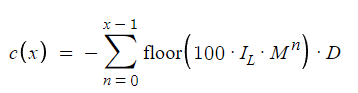
The equation illustrates the maximum possible drawdown. To clarify, if the cycle ends at the 10th order, the maximum drawdown would be the amount very close to the loss if the 10th order had gone as a losing trade. This is shown in the equation as 'n' goes from 0 to 'x-1', whereas previously 'n' was going from 0 to 'x-2' for losses before a profit.

The equation presented defines the maximum potential drawdown, a crucial concept for understanding risk in this strategy. For example, suppose the cycle concludes at the 10th order. In this context, the maximum drawdown can be thought of as an amount that closely approximates the loss incurred if the 10th order had resulted in a loss. The drawdown calculation is encapsulated within the equation by the variable 'n' iterating from 0 to x-1. This section specifies the range used to calculate the drawdown. This is a departure from the previous method of calculating losses, which involved 'n' traversing a range from 0 to x-2, followed by a profit. This adjustment to the equation's parameters provides a more accurate representation of the strategy's risk profile by accounting for the maximum possible loss scenario before a potential profit is realized.

To determine the maximum possible drawdown using our default input parameters, we closely observe how the values of the newly introduced variable adjust with changes in 'x'. This step is crucial for understanding the direct impact of varying 'x' on the potential drawdown, providing insights into the risk associated with different scenarios under our strategy.

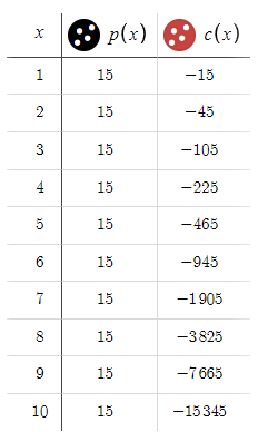
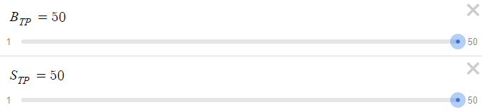
Given that we conclude the cycle with a win on the 10th order, we're looking at a maximum drawdown of $15,345 USD. This figure is considerably substantial, especially when contrasted with the relatively modest reward of $15 USD. Considering these dynamics, Let's increase the BTP and STP from 15 pips to 50 pips,

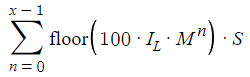
Now let's see how that turned out,

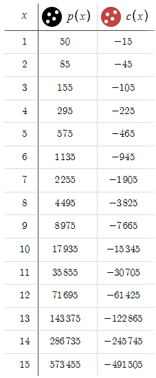
This represents a significant shift from our previous scenario, where our losses were increasing exponentially. Now, we find ourselves in a position where we are consistently achieving gains, highlighting a highly favorable risk-reward ratio. With such encouraging outcomes, it prompts the question: why limit ourselves to a 50 pips target? Let's explore the potential of extending our aim to 100 pips.

Notice a key observation here: the values of c(x) remain unchanged, while p(x) has increased over all values of x. This disparity might catch the eye of any observer, given the significant advantage in potential gains over losses. However, one must wonder about the underlying trap. To unravel this, consider if both the BTP and the STP were set at, say, 10,000 pips. Under such circumstances, it would take an eternity for the price to reach these targets. This leads us to a critical insight: the higher the BTP and STP, the lower the chances of completing the cycle, i.e. reaching either the BTP or the STP. In essence, this introduces a hidden element that we'll call "p," which represents the probability that a cycle will be completed given x. Indiscriminately increasing the BTP and STP decreases "p," and the lower "p" is, the less likely it is that the cycle will be completed. Therefore, regardless of the profit potential, if 'p' is minimal, the expected profits may never materialize. Since we're mainly dealing with the EURUSD, where a fluctuation of 100 pips is already significant, we've applied a provisional limit of 50 pips to both BTP and STP. This limit is based on intuition and can be adjusted as needed to effectively balance risk and reward.

Accounting for "p" and calculating our expected profit is a complex challenge. While mathematical optimization provides a structured approach, it alone cannot determine 'p' - the probability of cycle completion - which requires chart analysis for a more detailed understanding. Further complications arise because p is inherently unstable and behaves as a random variable. It's important to recognize that 'p' represents a vector of probability values, with each element indicating the probability of the cycle closing after a certain number of total orders. For example, the first element of the vector represents the probability of completing the cycle with only one order, and this logic extends to other elements for different order totals. A comprehensive examination of this concept, especially its application and implications, will be a key focus as we transition to code-based optimization in the next installment of this series.

In our analysis, we have overlooked an important factor: the spread. The spread plays a pivotal role in our strategy, affecting both profits and losses. To account for this, we adjust our calculations by subtracting certain terms from both p(x) and c(x) to include the spread in our analysis.

It's important to note that our adjustment takes into account all trades, from zero to x-1, recognizing that the spread affects every trade, whether profitable or not. For simplicity, we're currently treating the spread (denoted as S) as a constant value. This decision is made to avoid complicating our mathematical analysis with the added variability of a fluctuating spread. Although this simplification limits the realism of our model, it allows us to focus on the core aspects of our strategy without getting bogged down by excessive complexity.

Now that we have introduced s(x) into our calculations, we want to quantify the real impact of the spread on our profits. The effects are quite significant, with the spread-related losses escalating as x increases, potentially reaching up to 32,000 pips, or about $3,200. This adjustment not only reduces our potential profits by s(x), but also increases our potential losses by the same amount, significantly altering our risk-reward ratio. This shift highlights the critical importance of considering the spread in our strategic planning and underscores the need for careful management of this factor in optimizing our hedging strategy.

Coming to our final task, when we talk about "cutting down the cases for brute force," we're referring to the process of selectively eliminating certain parameter combinations that are unlikely to yield beneficial results for our strategy. This step is critical to optimizing our approach, especially when preparing for code-based optimization, because it allows us to focus our computational resources on exploring the most promising configurations.

For example, let's consider a scenario where we set the parameters BTP (Buy Trigger Point), STP (Sell Trigger Point), and D (Distance) all to 15, with M (Multiplier) at 1.5.

When we analyze the results of these settings, we quickly realize that such parameters lead to unsatisfactory results. Therefore, it's obvious that incorporating these specific values into our strategy or further optimization efforts would be futile.

The question then becomes, how do we proactively identify and eliminate such ineffective parameter combinations? While my initial discovery of these parameters was serendipitous, systematically identifying and eliminating all suboptimal inputs is a significant challenge. This requires a methodical approach, possibly including a preliminary analysis to assess the feasibility of different parameter sets before committing to full-scale brute-force optimization. In this way, we can streamline the optimization process and ensure that we only spend our efforts exploring parameter combinations that hold promise for improving the effectiveness of our trading strategy.

Addressing the challenge of systematically identifying and eliminating suboptimal parameter combinations in our optimization process is a complex task that we'll tackle in subsequent installments of this series. This approach will ensure a focused and efficient exploration of the most promising strategies, thereby increasing the overall effectiveness of our trading methodology. With that, we will stop here and continue in the next part.

Conclusion

In this third installment of our series, we began a deeper exploration into optimizing the Simple Hedge strategy, mostly delving into mathematical analysis and getting a basic idea of the brute force approach that we will do in the next part.

Looking ahead, subsequent articles in this series will move from theoretical exploration to practical code-based optimization, applying the principles and insights gained thus far to real-world trading scenarios. This shift promises to bring our strategy into sharper focus, offering tangible improvements and actionable strategies for traders seeking to maximize returns while effectively managing risk.

Your participation and feedback have been invaluable throughout this series, and I encourage you to continue to share your thoughts and suggestions as we move forward. Together, we're not just optimizing a trading strategy; we're paving the way for more informed, effective trading decisions that can stand the test of market volatility and uncertainty.

Happy Coding! Happy Trading!