价格行为分析工具包开发(第二十部分):外部资金流(4)——相关性路径探索器

内容
概述
外汇交易需要对诸多因素有清晰的理解。其中一个关键因素就是货币相关性。货币相关性指的是两对货币相对彼此的走势情况。它表明这两对货币是同向变动、反向变动,还是随时间推移而随机变动。由于货币总是以货币对的形式进行交易,所以每一对货币都与其他货币对相关联,从而形成了一个相互依存的网络。
了解这些关系能够优化您的交易策略并降低风险。例如,在两对货币高度正相关时期同时买入欧元兑美元和英镑兑美元,会使您面临相同市场力量的影响加倍,进而增加风险。反之,这种了解能让交易者构建多元化的投资组合,并有效实施套期保值策略。
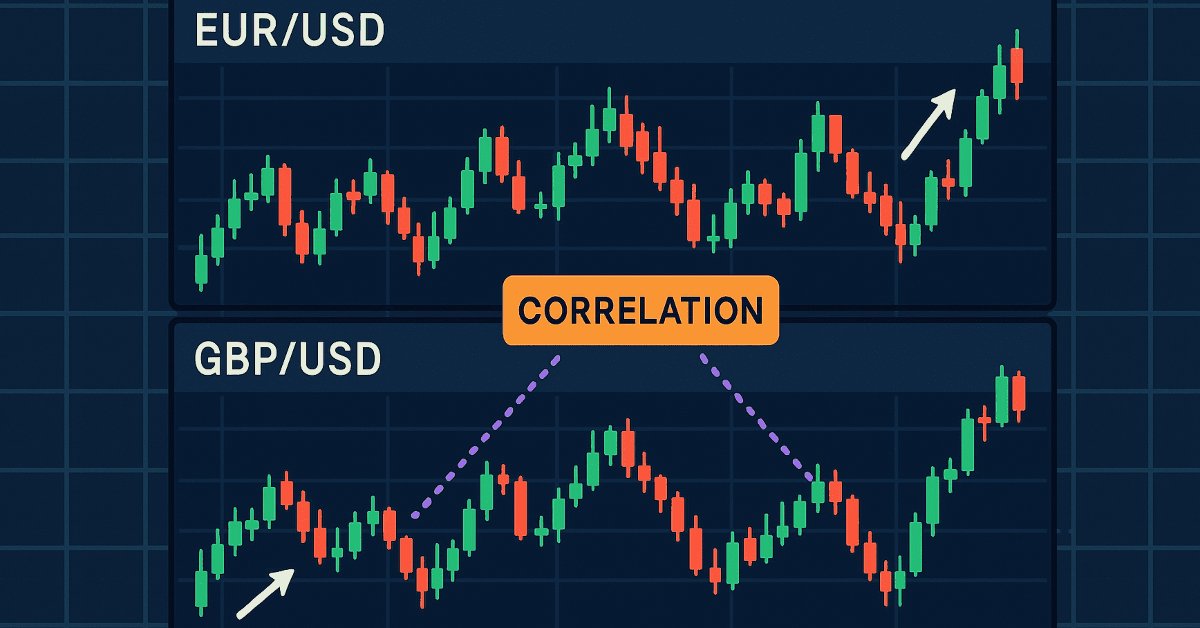
本文将阐述如何将货币相关性分析纳入您的交易工具包。其提供了实用的见解和可操作的策略,以提升交易表现。以下两张图表展示了同一日期欧元兑美元和英镑兑美元的市场结构。4月2日,这两对货币均呈看涨态势,而4月3日则均转为看跌,这体现了它们之间的正相关性。交易者可以利用其中一对货币的走势来确认另一对货币的反转信号。例如,如果欧元兑美元处于超买状态,而英镑兑美元正在下跌,这就为欧元兑美元可能出现反转提供了明确信号。相关性路径探索器工具至关重要,因为它能清晰展示货币对之间的相互关系,帮助交易者更准确地把握市场动态。
英镑兑美元

图例1. 英镑兑美元
欧元兑美元

图例2. 欧元兑美元
系统概况
货币相关性通过一个介于-1到+1之间的系数来表示。系数值接近+1表明货币对倾向于同向变动,而系数值接近-1则表明它们反向变动。系数值接近零则表示两者之间几乎没有或不存在关联。
这种认知对于有效的风险管理至关重要。例如,在货币对呈现强烈正相关性的时期同时买入欧元兑美元和英镑兑美元,会使整体市场风险敞口增加,实际上相当于风险加倍。相反,正如我之前提到的,了解相关性的程度能让交易者实现投资组合多元化,并运用套期保值策略来防范意外的市场波动。
该系统由两个相互关联的组件构成。第一个组件是MQL5 EA,它持续获取欧元兑美元和英镑兑美元的历史价格数据。该系统将这些数据打包成JSON结构,并发送至一个Python服务器。第二个组件是一个基于Python的分析引擎。它使用Pandas库计算整体相关性和滚动相关性,并利用Matplotlib库生成固定宽度的滚动相关性图表。此外,该服务器还会生成清晰的评论,解释货币对是同向变动还是出现分歧,并阐述这对交易策略的影响。
通过查看以下流程图,可进一步了解该系统的数据流和分析过程。

图例3. 流程图
本图以清晰直观的方式呈现了系统的工作流程,从MetaTrader 5中的数据检索,到Python服务器上生成分析结果和评论的整个过程。图中标记为A至H的节点代表了流程中的各个步骤,展示了数据如何被收集、打包成JSON格式、传输至服务器、用Pandas解析和分析、用Matplotlib可视化,并最终附上解释性评论后返回分析结果。
技术细节
MQL5 EA
数据提取
EA使用MetaTrader 5内置的函数CopyRates()来检索历史价格数据。该函数获取一个价格记录数组(结构化为MqlRates),其中包含给定交易品种和时间框架下的时间、开盘价、最高价、最低价和收盘价等信息。在该EA中,用户可以使用参数BarsToExport来配置时间框架(例如,通过PERIOD_M15设置15分钟间隔)和要导出的K线数量(数据点)。由于可配置这些值,该EA可以适应各种交易策略。无论交易者需要短期说明还是对历史趋势的更广泛视角。
MqlRates rates1[];
if(CopyRates(Symbol1, TimeFrame, 0, BarsToExport, rates1) <= 0)
{
   Print("Failed to copy rates for ", Symbol1);
   return "";
}
ArraySetAsSeries(rates1, true);
一旦获取了每个货币对(如欧元兑美元和英镑兑美元)的数据,EA会确保将数据数组设置为序列形式。这一步骤至关重要,因为它对数组进行排列,使最新K线位于索引0处,这与MQL5环境中许多其他函数期望的数据格式相一致。这种历史数据的准备过程确保了获取到正确数量的K线,并保持了恰当的时间顺序,这对于后续的分析至关重要。
JSON负载构建
收集完价格数据后,EA会构建一个JSON负载,将数据整齐地组织成结构化格式以便传输。BuildJSONPayload()函数首先创建一个包含两个货币对名称的JSON对象。然后,针对每个货币对,该函数构建一个数据对象数组。数组中的每个对象代表一K线历史数据,并包含两个关键信息:时间(使用TimeToString()函数,并配合参数 TIME_DATE和TIME_SECONDS进行统一格式化)和收盘价(使用DoubleToString()函数格式化为五位小数)。
string json = "{";
json += "\"symbol1\":\"" + Symbol1 + "\",";
json += "\"symbol2\":\"" + Symbol2 + "\",";
json += "\"data1\":[";
for(int i = 0; i < ArraySize(rates1); i++)
{
   string timeStr = TimeToString(rates1[i].time, TIME_DATE | TIME_SECONDS);
   json += "{\"time\":\"" + timeStr + "\",\"close\":" + DoubleToString(rates1[i].close, 5) + "}";
   if(i < ArraySize(rates1) - 1)
      json += ",";
}
json += "],";
// The same pattern repeats for Symbol2's data array.
json += "}";
return json;
这种模块化的方法确保了负载中包含供Python服务器分析所需的所有详细信息。JSON结构使得数据更易于保持一致性,并确保服务器能够无误地解析数据。例如,通过将数组标记为data1和data2,服务器脚本就能准确地知道哪个数据集对应哪个货币对。这种清晰的分隔对于后续计算相关性时合并数据至关重要。该函数会遍历每个历史数据数组,用恰当的JSON格式拼接每条记录,然后通过闭合JSON对象来完成负载构建。
WebRequest集成
一旦构建好JSON负载,EA就会使用MetaTrader的WebRequest()函数发送数据,该函数是从交易平台直接执行HTTP请求的重要工具。这个组件负责处理MQL5 EA与执行进一步分析的Python服务器之间的通信。在发送数据之前,智能交易系统会使用StringToCharArray()函数将JSON字符串转换为动态uchar数组,因为WebRequest()以这种格式接受请求体。这种转换是必要的,以确保负载能够通过网络正确传输。
string requestHeaders = "Content-Type: application/json\r\n";
uchar result[];
string responseHeaders;
int webRequestResult = WebRequest("POST", pythonUrl, requestHeaders, timeout, requestData, result, responseHeaders);
if(webRequestResult == -1)
{
   Print("Error in WebRequest. Error code = ", GetLastError());
   return;
}

string response = CharArrayToString(result);
Print("Server response: ", response);
随后,EA会设置HTTP请求头,通过“Content-Type: application/json\r\n”请求头指明数据为JSON格式。诸如pythonUrl(服务器端点)和超时时长(EA等待响应的时间)等可配置的输入项,使用户能够根据自身环境对网络参数进行微调。使用这些请求头和超时设置,通过WebRequest()函数向Python服务器发送HTTP POST请求。如果请求失败,智能交易系统会打印错误代码,这有助于排查连接问题。否则,它会将返回的uchar数组响应转换回字符串,然后打印服务器的响应——该响应预计会包含有用信息,例如由Python分析引擎计算出的相关系数值以及生成的任何评论。
Python分析服务器
服务器环境
该系统基于Flask服务器构建,用于监听POST请求。启动时,服务器使用Flask的默认设置进行初始化,并将日志级别设置为DEBUG。这种配置确保所有传入的请求和处理步骤都会被详细记录。该服务器旨在接收JSON数据,对其进行处理,执行分析,并以JSON格式返回结果。通过使用Flask,服务器保持轻量级和高效性,能够在无图形用户界面(GUI)的后台环境中处理Web请求,非常适合自动化交易应用。
import matplotlib
matplotlib.use("Agg")  # Use non-interactive backend to avoid GUI overhead
import matplotlib.pyplot as plt
from flask import Flask, request, jsonify
import logging

app = Flask(__name__)
logging.basicConfig(level=logging.DEBUG)

if __name__ == "__main__":
    app.run(host="127.0.0.1", port=5000)
数据解析与分析
服务器收到POST请求后,首先尝试解析传入的JSON负载。如果默认解析器解析失败,代码会对原始请求数据进行解码,去除最后一个闭合大括号之后的任何多余字符,然后加载JSON数据。解析后的数据随后被转换为两个独立的Pandas数据框(DataFrames),每个货币对对应一个数据框。从负载中提取的“时间”字段会被解析并转换为日期时间对象,以便进行准确的合并和时序分析。在根据共同的“时间”列合并这两个数据框后,服务器会计算两个关键的相关性指标。首先,计算两个交易品种收盘价之间的整体相关性。其次,计算一个窗口为50根K线的滚动相关性。这种滚动相关性能够揭示两对货币对之间的相关性如何随时间变化,这对于理解市场动态以及发现两对货币对关系增强或减弱的时期至关重要。
import pandas as pd
import json

@app.route('/analyze', methods=['POST'])
def analyze():
    # Parse JSON payload
    data = request.get_json(silent=True)
    if not data:
        raw_data = request.data.decode('utf-8').strip()
        app.logger.debug("Raw request data: %s", raw_data)
        try:
            end_index = raw_data.rfind("}")
            trimmed_data = raw_data[:end_index+1] if end_index != -1 else raw_data
            data = json.loads(trimmed_data)
        except Exception as e:
            app.logger.error("Failed to parse JSON: %s", str(e))
            return jsonify({"error": "Invalid JSON received"}), 400

    # Convert incoming JSON arrays to DataFrames
    data1 = pd.DataFrame(data["data1"])
    data2 = pd.DataFrame(data["data2"])

    # Convert time strings to datetime objects
    data1['Time'] = pd.to_datetime(data1['time'])
    data2['Time'] = pd.to_datetime(data2['time'])

    # Merge DataFrames on 'Time'
    merged = pd.merge(data1, data2, on="Time",
                      suffixes=('_' + data["symbol1"], '_' + data["symbol2"]))

    # Calculate overall correlation between the close prices
    correlation = merged[f'close_{data["symbol1"]}'].corr(merged[f'close_{data["symbol2"]}'])

    # Calculate rolling correlation with a 50-bar window
    merged['RollingCorrelation'] = merged[f'close_{data["symbol1"]}'].rolling(window=50).corr(merged[f'close_{data["symbol2"]}'])

    # [Graph generation and commentary code follows here, see next sections]
图表生成与存储
为了实现可视化展示,服务器采用Matplotlib库,并使用“Agg”后端。该后端无需图形用户界面,确保在无界面环境中生成图表,且不会触发任何与图形用户界面相关的额外开销。图表以固定尺寸生成,宽度设为7.5英寸,分辨率为100DPI。这种配置保证了输出图像的固定宽度为750像素,使得报告中的输出图像保持一致,便于快速解读可视化数据。一旦生成,显示滚动相关性的图表将以PNG文件形式保存在与Python脚本相同的目录下。将图像本地存储便于轻松检索和进一步分享,而无需在服务器的JSON响应中包含实际图形。
import matplotlib.pyplot as plt

# Generate a rolling correlation plot
plt.figure(figsize=(7.5, 6), dpi=100)  # 7.5 inches * 100 dpi = 750 pixels width
plt.plot(merged['Time'], merged['RollingCorrelation'], label="Rolling Correlation (50 bars)")
plt.xlabel("Time")
plt.ylabel("Correlation")
plt.title(f"{data['symbol1']} and {data['symbol2']} Rolling Correlation")
plt.legend()
plt.grid(True)
plt.tight_layout()

# Save the graph as a PNG file in the same folder
plot_filename = "rolling_correlation.png"
plt.savefig(plot_filename)
plt.close()
解读性评述
除了原始数据和图表外,服务器还通过生成解读性评述来增强分析效果。这种评述由一个专门设计的函数生成,该函数会同时考察整体相关性和近期(滚动)相关性数值。例如,如果整体相关性非常高(接近+1),评述会解释这两个货币对通常同步波动,这可能表明在交易多个货币对时,分散投资的效果有限。反之,如果相关性较低或变为负值,评述则会强调货币对出现背离的潜在可能,以及进行对冲或调整头寸的机会。
def generate_commentary(corr, rolling_series):
    """Generate a commentary based on overall and recent correlation values."""
    commentary = ""
    if corr >= 0.8:
        commentary += ("The currency pairs have a very strong positive correlation, meaning "
                       "they typically move together. This may support the use of hedging strategies.\n")
    elif corr >= 0.5:
        commentary += ("The pairs display a moderately strong positive correlation with some deviations, "
                       "indicating they often move in the same direction.\n")
    elif corr >= 0.0:
        commentary += ("The overall correlation is weakly positive, suggesting occasional movement together "
                       "but limited consistency, which may offer diversification opportunities.\n")
    elif corr >= -0.5:
        commentary += ("The pairs exhibit a weak to moderate negative correlation; they tend to move in opposite "
                       "directions, which can be useful for diversification.\n")
    else:
        commentary += ("The pairs have a strong negative correlation, implying they generally move in opposite "
                       "directions, a factor exploitable in hedging strategies.\n")

    if not rolling_series.empty:
        recent_trend = rolling_series.iloc[-1]
        commentary += f"Recently, the rolling correlation is at {recent_trend:.2f}. "
        if recent_trend > 0.8:
            commentary += ("This high correlation suggests near mirror-like movement. "
                           "Relative strength approaches may need reconsideration for diversification.")
        elif recent_trend < 0.3:
            commentary += ("A significant drop in correlation indicates potential decoupling. "
                           "This may signal opportunities in pair divergence trades.")
        else:
            commentary += ("The correlation remains moderate, meaning the pairs show some synchronization but also "
                           "retain independent movement.")
    return commentary
该评述还就近期相关性趋势提供见解,为交易者提供实用指导,帮助他们理解这些统计信号对风险管理和交易策略可能意味着什么。通过将定量分析与定性见解相结合,该系统帮助交易者更好地理解市场行为,并做出更明智的决策。
成果
在深入探讨成果之前,有必要说明如何启动Python服务器。首先,从python.org下载并安装Python,然后运行 python -m venv venv 创建一个虚拟环境并激活。接下来,通过执行pip install Flask pandas matplotlib安装所需的软件包。创建一个Python脚本(例如,server.py),其中包含你的Flask服务器代码和必要的端点。最后,导航到脚本所在目录,并运行python server.py启动服务器。有关外部流程的更多详细信息,请参阅我之前的一篇文章 。
以下是对欧元兑美元和英镑兑美元货币对进行的测试成果展示。为获得最佳效果,请确保在您的EA中指定的相同货币对,用来测试该系统。最初,命令提示符日志显示系统已成功初始化,并清楚地显示了MQL5 EA从MetaTrader 5传输到Python服务器的数据——这包括4月2日至4月9日期间的开盘价、收盘价和时间值。日志条目"POST /analyze HTTP/1.1" 200确认了连接成功,并且Python服务器按预期执行了所需的处理。
DEBUG:plotter:Raw request data: {"symbol1":"EURUSD","symbol2":"GBPUSD","data1":[{"time":"2025.04.09 07:00:00"
,"close":1.10766},{"time":"2025.04.09 06:45:00","close":1.10735},{"time":"2025.04.09 06:30:00","close":1.10602}
,{"time":"2025.04.09 06:15:00","close":1.10538},{"time":"2025.04.09 06:00:00","close":1.10486},
{"time":"2025.04.09 05:45:00","close":1.10615},{"time":"2025.04.09 05:30:00","close":1.10454},
{"time":"2025.04.09 05:15:00","close":1.10402},{"time":"2025.04.09 05:00:00","close":1.10447},
{"time":"2025.04.09 04:45:00","close":1.10685},{"time":"2025.04.09 04:30:00","close":1.10582},
{"time":"2025.04.09 04:15:00","close":1.10617},{"time":"2025.04.09 04:00:00","close":1.10384},
{"time":"2025.04.09 03:45:00","close":1.10196},{"time":"2025.04.09 03:30:00","close":1.10184},
{"time":"2025.04.09 03:15:00","close":1.10339},{"time":"2025.04.09 03:00:00","close":1.10219},
{"time":"2025.04.09 02:45:00","close":1.10197},{"time":"2025.04.09 02:30:00","close":1.10130},
{"time":"2025.04.09 02:15:00","close":1.10233},{"time":"2025.04.09 02:00:00","close":1.10233},
{"time":"2025.04.09 01:45:00","close":1.10200},{"time":"2025.04.09 01:30:00","close":1.10289},
{"time":"2025.04.09 01:15:00","close":1.10382},{"time":"2025.04.09 01:00:00","close":1.10186},
{"time":"2025.04.09 00:45:00","close":1.10148},{"time":"2025.04.09 00:30:00","close":1.09985},
{"time":"2025.04.09 00:15:00","close":1.09894},{"time":"2025.04.09 00:00:00","close":1.09747},
{"time":"2025.04.08 23:45:00","close":1.09776},{"time":"2025.04.08 23:30:00","close":1.09789},
{"time":"2025.04.08 23:15:00","close":1.09793},{"time":"2025.04.08 23:00:00","close":1.09740},
{"time":"2025.04.08 22:45:00","close":1.09681},{"time":"2025.04.08 22:30:00","close":1.09718},
{"time":"2025.04.08 22:15:00","close":1.09669},{"time":"2025.04.08 22:00:00","close":1.09673},
{"time":"2025.04.08 21:45:00","close":1.09586},{"time":"2025.04.08 21:30:00","close":1.09565},
{"time":"2025.04.08 21:15:00","close":1.09507},{"time":"2025.04.08 21:00:00","close":1.09493},
{"time":"2025.04.08 20:45:00","close":1.09529},{"time":"2025.04.08 20:30:00","close":1.09442},
{"time":"2025.04.08 20:15:00","close":1.09417},{"time":"2025.04.08 20:00:00","close":1.09533},
{"time":"2025.04.08 19:45:00","close":1.09541},{"time":"2025.04.08 19:30:00","close":1.09587},
{"time":"2025.04.08 19:15:00","close":1.09684},{"time":"2025.04.08 19:00:00","close":1.09724},
{"time":"2025.04.08 18:45:00","close":1.09521},{"time":"2025.04.08 18:30:00","close":1.09551},
{"time":"2025.04.08 18:15:00","close":1.09561},{"time":"2025.04.08 18:00:00","close":1.09474},
{"time":"2025.04.08 17:45:00","close":1.09337},{"time":"2025.04.08 17:30:00","close":1.09334},
{"time":"2025.04.08 17:15:00","close":1.09421},{"time":"2025.04.08 17:00:00","close":1.09429},
{"time":"2025.04.08 16:45:00","close":1.09296},{"time":"2025.04.08 16:30:00","close":1.09210},
{"time":"2025.04.08 16:15:00","close":1.09123},{"time":"2025.04.08 16:00:00","close":1.09073},
{"time":"2025.04.08 15:45:00","close":1.09116},{"time":"2025.04.08 15:30:00","close":1.09083},
{"time":"2025.04.08 15:15:00","close":1.09119},{"time":"2025.04.08 15:00:00","close":1.08986},
{"time":"2025.04.08 14:45:00","close":1.09102},{"time":"2025.04.08 14:30:00","close":1.08954},
{"time":"2025.04.08 14:15:00","close":1.09051},{"time":"2025.04.08 14:00:00","close":1.09213},
{"time":"2025.04.08 13:45:00","close":1.09357},{"time":"2025.04.08 13:30:00","close":1.09300},
{"time":"2025.04.08 13:15:00","close":1.09548},{"time":"2025.04.08 13:00:00","close":1.09452},
{"time":"2025.04.08 12:45:00","close":1.09485},{"time":"2025.04.08 12:30:00","close":1.09585},
{"time":"2025.04.08 12:15:00","close":1.09477},{"time":"2025.04.08 12:00:00","close":1.09512},
{"time":"2025.04.08 11:45:00","close":1.09342},{"time":"2025.04.08 11:30:00","close":1.09311},
{"time":"2025.04.07 09:45:00","close":1.09627},{"time":"2025.04.07 09:30:00","close":1.09545},
{"time":"2025.04.07 09:15:00","close":1.09597},{"time":"2025.04.07 09:00:00","close":1.09729},
{"time":"2025.04.07 08:45:00","close":1.09918},{"time":"2025.04.07 08:30:00","close":1.09866},
{"time":"2025.04.07 08:15:00","close":1.09705},{"time":"2025.04.07 08:00:00","close":1.10051},
{"time":"2025.04.07 07:45:00","close":1.10006},{"time":"2025.04.07 07:30:00","close":1.10232},
{"time":"2025.04.07 07:15:00","close":1.10273},{"time":"2025.04.07 07:00:00","close":1.10397},
{"time":"2025.04.07 06:45:00","close":1.10029},{"time":"2025.04.07 06:30:00","close":1.10083},
{"time":"2025.04.07 06:15:00","close":1.10012},{"time":"2025.04.07 06:00:00","close":1.10084},
{"time":"2025.04.07 05:45:00","close":1.10183},{"time":"2025.04.07 05:30:00","close":1.09905},
{"time":"2025.04.07 05:15:00","close":1.09941},{"time":"2025.04.07 05:00:00","close":1.09826},
{"time":"2025.04.07 04:45:00","close":1.09848},{"time":"2025.04.07 04:30:00","close":1.09830},
{"time":"2025.04.07 04:15:00","close":1.09739},{"time":"2025.04.07 04:00:00","close":1.09608},
{"time":"2025.04.07 03:45:00","close":1.09503},{"time":"2025.04.07 03:30:00","close":1.09456},
{"time":"2025.04.07 03:15:00","close":1.09373},{"time":"2025.04.07 03:00:00","close":1.09343},
{"time":"2025.04.07 02:45:00","close":1.09353},{"time":"2025.04.07 02:30:00","close":1.09248},
{"time":"2025.04.07 02:15:00","close":1.09360},{"time":"2025.04.07 02:00:00","close":1.09550},
{"time":"2025.04.07 01:45:00","close":1.09673},{"time":"2025.04.07 01:30:00","close":1.09740},
{"time":"2025.04.07 01:15:00","close":1.09688},{"time":"2025.04.07 01:00:00","close":1.09649},
{"time":"2025.04.07 00:45:00","close":1.09667},{"time":"2025.04.07 00:30:00","close":1.09526},
{"time":"2025.04.07 00:15:00","close":1.09555},{"time":"2025.04.07 00:00:00","close":1.09517},
{"time":"2025.04.06 23:45:00","close":1.09825},{"time":"2025.04.06 23:30:00","close":1.09981},
{"time":"2025.04.06 23:15:00","close":1.09872},{"time":"2025.04.06 23:00:00","close":1.09981},
{"time":"2025.04.06 22:45:00","close":1.09822},{"time":"2025.04.06 22:30:00","close":1.09803},
{"time":"2025.04.06 22:15:00","close":1.09826},{"time":"2025.04.06 22:00:00","close":1.09529},
{"time":"2025.04.06 21:45:00","close":1.09147},{"time":"2025.04.06 21:30:00","close":1.09046},
{"time":"2025.04.06 21:15:00","close":1.08910},{"time":"2025.04.06 21:00:00","close":1.08818},
{"time":"2025.04.04 20:45:00","close":1.09623},{"time":"2025.04.04 20:30:00","close":1.09435},
{"time":"2025.04.04 20:15:00","close":1.09339},{"time":"2025.04.04 20:00:00","close":1.09502},
{"time":"2025.04.04 19:45:00","close":1.09436},{"time":"2025.04.04 19:30:00","close":1.09631},
{"time":"2025.04.04 19:15:00","close":1.09425},{"time":"2025.04.04 19:00:00","close":1.09358},
{"time":"2025.04.04 18:45:00","close":1.09447},{"time":"2025.04.04 18:30:00","close":1.09611},
{"time":"2025.04.04 18:15:00","close":1.09604},{"time":"2025.04.04 18:00:00","close":1.09531},
{"time":"2025.04.04 17:45:00","close":1.09472},{"time":"2025.04.04 17:30:00","close":1.09408},
{"time":"2025.04.04 17:15:00","close":1.09311},{"time":"2025.04.04 17:00:00","close":1.09407},
{"time":"2025.04.04 16:45:00","close":1.09714},{"time":"2025.04.04 16:30:00","close":1.09690},
{"time":"2025.04.04 16:15:00","close":1.09845},{"time":"2025.04.04 16:00:00","close":1.09892},
{"time":"2025.04.04 15:45:00","close":1.10139},{"time":"2025.04.04 15:30:00","close":1.09998},
{"time":"2025.04.04 15:15:00","close":1.09837},{"time":"2025.04.04 15:00:00","close":1.09970},
{"time":"2025.04.04 14:45:00","close":1.09862},{"time":"2025.04.04 14:30:00","close":1.09706},
{"time":"2025.04.04 14:15:00","close":1.09991},{"time":"2025.04.04 14:00:00","close":1.10068},
{"time":"2025.04.04 13:45:00","close":1.10057},{"time":"2025.04.04 13:30:00","close":1.10252},
{"time":"2025.04.04 13:15:00","close":1.10288},{"time":"2025.04.04 13:00:00","close":1.10358},
{"time":"2025.04.04 12:45:00","close":1.10200},{"time":"2025.04.04 12:30:00","close":1.10289},
{"time":"2025.04.04 12:15:00","close":1.10794},{"time":"2025.04.04 12:00:00","close":1.10443},
{"time":"2025.04.04 11:45:00","close":1.10601},{"time":"2025.04.04 11:30:00","close":1.10697},
{"time":"2025.04.04 11:15:00","close":1.10502},{"time":"2025.04.04 11:00:00","close":1.10517},
{"time":"2025.04.04 10:45:00","close":1.10305},{"time":"2025.04.04 10:30:00","close":1.10340},
{"time":"2025.04.04 10:15:00","close":1.10447},{"time":"2025.04.04 10:00:00","close":1.09869},
{"time":"2025.04.04 09:45:00","close":1.09844},{"time":"2025.04.04 09:30:00","close":1.09757},
{"time":"2025.04.04 09:15:00","close":1.09820},{"time":"2025.04.04 09:00:00","close":1.09786},
{"time":"2025.04.04 08:45:00","close":1.09962},{"time":"2025.04.04 08:30:00","close":1.10002},
{"time":"2025.04.04 08:15:00","close":1.10062},{"time":"2025.04.04 08:00:00","close":1.10034},
{"time":"2025.04.04 07:45:00","close":1.10042},{"time":"2025.04.04 07:30:00","close":1.10223},
{"time":"2025.04.04 07:15:00","close":1.10490},{"time":"2025.04.04 07:00:00","close":1.10641},
{"time":"2025.04.04 06:45:00","close":1.10506},{"time":"2025.04.04 06:30:00","close":1.10638},
{"time":"2025.04.04 06:15:00","close":1.10649},{"time":"2025.04.04 06:00:00","close":1.10747},
{"time":"2025.04.04 05:45:00","close":1.10843},{"time":"2025.04.04 05:30:00","close":1.10809},
{"time":"2025.04.04 05:15:00","close":1.11057},{"time":"2025.04.04 05:00:00","close":1.10984},
{"time":"2025.04.04 04:45:00","close":1.10874},{"time":"2025.04.04 04:30:00","close":1.10896},
{"time":"2025.04.04 04:15:00","close":1.10906},{"time":"2025.04.04 04:00:00","close":1.10876},
{"time":"2025.04.04 03:45:00","close":1.10937},{"time":"2025.04.04 03:30:00","close":1.10918},
{"time":"2025.04.04 03:15:00","close":1.10766},{"time":"2025.04.04 03:00:00","close":1.10695},
{"time":"2025.04.04 02:45:00","close":1.10632},{"time":"2025.04.04 02:30:00","close":1.10668},
{"time":"2025.04.04 02:15:00","close":1.10625},{"time":"2025.04.04 02:00:00","close":1.10773},
{"time":"2025.04.04 01:45:00","close":1.10677},{"time":"2025.04.04 01:30:00","close":1.10625},
{"time":"2025.04.04 01:15:00","close":1.10610},{"time":"2025.04.04 01:00:00","close":1.10589},
{"time":"2025.04.04 00:45:00","close":1.10606},{"time":"2025.04.04 00:30:00","close":1.10603},
{"time":"2025.04.04 00:15:00","close":1.10403},{"time":"2025.04.04 00:00:00","close":1.10432},
{"time":"2025.04.03 23:45:00","close":1.10452},{"time":"2025.04.03 23:30:00","close":1.10467},
{"time":"2025.04.03 23:15:00","close":1.10446},{"time":"2025.04.03 23:00:00","close":1.10524},
{"time":"2025.04.03 22:45:00","close":1.10642},{"time":"2025.04.03 22:30:00","close":1.10631},
{"time":"2025.04.03 22:15:00","close":1.10582},{"time":"2025.04.03 22:00:00","close":1.10577},
{"time":"2025.04.03 21:45:00","close":1.10515},{"time":"2025.04.03 21:30:00","close":1.10497},
{"time":"2025.04.03 21:15:00","close":1.10505},{"time":"2025.04.03 21:00:00","close":1.10488},
{"time":"2025.04.03 20:45:00","close":1.10514},{"time":"2025.04.03 20:30:00","close":1.10448},
{"time":"2025.04.03 20:15:00","close":1.10312},{"time":"2025.04.03 20:00:00","close":1.10253},
{"time":"2025.04.03 19:45:00","close":1.10275},{"time":"2025.04.03 19:30:00","close":1.10164},
{"time":"2025.04.03 19:15:00","close":1.10192},{"time":"2025.04.03 19:00:00","close":1.10320},
{"time":"2025.04.03 18:45:00","close":1.10373},{"time":"2025.04.03 18:30:00","close":1.10362},
{"time":"2025.04.03 18:15:00","close":1.10322},{"time":"2025.04.03 18:00:00","close":1.10236},
{"time":"2025.04.03 17:45:00","close":1.10245},{"time":"2025.04.03 17:30:00","close":1.10222},
{"time":"2025.04.03 17:15:00","close":1.10273},{"time":"2025.04.03 17:00:00","close":1.10267},
{"time":"2025.04.03 16:45:00","close":1.10386},{"time":"2025.04.03 16:30:00","close":1.10404},
{"time":"2025.04.03 16:15:00","close":1.10367},{"time":"2025.04.03 16:00:00","close":1.10491},
{"time":"2025.04.03 15:45:00","close":1.10506},{"time":"2025.04.03 15:30:00","close":1.10452},
{"time":"2025.04.03 15:15:00","close":1.10613},{"time":"2025.04.03 15:00:00","close":1.10922},
{"time":"2025.04.03 14:45:00","close":1.11182},{"time":"2025.04.03 14:30:00","close":1.11197},
{"time":"2025.04.03 14:15:00","close":1.10950},{"time":"2025.04.03 14:00:00","close":1.10981},
{"time":"2025.04.03 13:45:00","close":1.10784},{"time":"2025.04.03 13:30:00","close":1.10911},
{"time":"2025.04.03 13:15:00","close":1.10943},{"time":"2025.04.03 13:00:00","close":1.11064},
{"time":"2025.04.03 12:45:00","close":1.10816},{"time":"2025.04.03 12:30:00","close":1.10910},
{"time":"2025.04.03 12:15:00","close":1.10858},{"time":"2025.04.03 12:00:00","close":1.10867},
{"time":"2025.04.03 11:45:00","close":1.10876},{"time":"2025.04.03 11:30:00","close":1.10839},
{"time":"2025.04.03 11:15:00","close":1.10570},{"time":"2025.04.03 11:00:00","close":1.10596},
{"time":"2025.04.03 10:45:00","close":1.10521},{"time":"2025.04.03 10:30:00","close":1.10696},
{"time":"2025.04.03 10:15:00","close":1.10859},{"time":"2025.04.03 10:00:00","close":1.11052},
{"time":"2025.04.03 09:45:00","close":1.10305},{"time":"2025.04.03 09:30:00","close":1.10280},
{"time":"2025.04.03 09:15:00","close":1.10336},{"time":"2025.04.03 09:00:00","close":1.10304},
{"time":"2025.04.03 08:45:00","close":1.10093},{"time":"2025.04.03 08:30:00","close":1.10092},
{"time":"2025.04.03 08:15:00","close":1.09885},{"time":"2025.04.03 08:00:00","close":1.09803},
{"time":"2025.04.03 07:45:00","close":1.09707},{"time":"2025.04.03 07:30:00","close":1.09658},
{"time":"2025.04.03 07:15:00","close":1.09497},{"time":"2025.04.03 07:00:00","close":1.09733},
{"time":"2025.04.03 06:45:00","close":1.09896},{"time":"2025.04.03 06:30:00","close":1.09775},
{"time":"2025.04.03 06:15:00","close":1.09488},{"time":"2025.04.03 06:00:00","close":1.09457},
{"time":"2025.04.03 05:45:00","close":1.09444},{"time":"2025.04.03 05:30:00","close":1.09515},
{"time":"2025.04.03 05:15:00","close":1.09431},{"time":"2025.04.03 05:00:00","close":1.09171},
{"time":"2025.04.03 04:45:00","close":1.09069},{"time":"2025.04.03 04:30:00","close":1.09104},
{"time":"2025.04.03 04:15:00","close":1.09109},{"time":"2025.04.03 04:00:00","close":1.09110},
{"time":"2025.04.03 03:45:00","close":1.09148},{"time":"2025.04.03 03:30:00","close":1.09118},
{"time":"2025.04.03 03:15:00","close":1.09196},{"time":"2025.04.03 03:00:00","close":1.09115},
{"time":"2025.04.03 02:45:00","close":1.09122},{"time":"2025.04.03 02:30:00","close":1.09207},
{"time":"2025.04.03 02:15:00","close":1.09220},{"time":"2025.04.03 02:00:00","close":1.09134},
{"time":"2025.04.03 01:45:00","close":1.09132},{"time":"2025.04.03 01:30:00","close":1.09137},
{"time":"2025.04.03 01:15:00","close":1.09078},{"time":"2025.04.03 01:00:00","close":1.08970},
{"time":"2025.04.03 00:45:00","close":1.08906},{"time":"2025.04.03 00:30:00","close":1.08995},
{"time":"2025.04.03 00:15:00","close":1.08831},{"time":"2025.04.03 00:00:00","close":1.08905},
{"time":"2025.04.02 23:45:00","close":1.09044},{"time":"2025.04.02 23:30:00","close":1.09068},
{"time":"2025.04.02 23:15:00","close":1.08874},{"time":"2025.04.02 23:00:00","close":1.08552},
{"time":"2025.04.02 22:45:00","close":1.08389},{"time":"2025.04.02 22:30:00","close":1.08277},
{"time":"2025.04.02 22:15:00","close":1.08221},{"time":"2025.04.02 22:00:00","close":1.08161},
{"time":"2025.04.02 21:45:00","close":1.08274},{"time":"2025.04.02 21:30:00","close":1.08286},
{"time":"2025.04.02 21:15:00","close":1.08156},{"time":"2025.04.02 21:00:00","close":1.08350},
{"time":"2025.04.02 20:45:00","close":1.08507},{"time":"2025.04.02 20:30:00","close":1.08184},
INFO:werkzeug:127.0.0.1 - - [09/Apr/2025 09:04:18] "POST /analyze HTTP/1.1" 200 -
以下是MetaTrader 5“Experts”选项卡中的日志,其中包含Python服务器对相关性分析的评述。日志详细记录了从前几天到当天的数据,展示了欧元兑美元和英镑兑美元这两组货币对彼此之间的波动关系。评述对相关性图表进行了解读,指出在记录期间,这两组货币对总体上保持较强的正相关性。
2025.04.09 00:57:33.296 Correlation Pathfinder (GBPUSD,M15)     Server response:
{"commentary":"The overall correlation is weakly positive, suggesting occasional movement together but
limited consistency, which may offer diversification opportunities.\nRecently, the rolling correlation is at
0.82. This high correlation suggests near mirror-like movement. Relative strength approaches may need
reconsideration for diversification.","correlation":0.3697032305325312,"message":"Plot saved as rolling_
correlation.png"}
这表明这两组货币对总体上倾向于同步波动,尽管有时也会出现细微偏差。这些偏差可能暗示市场出现暂时性分化,凸显了进行投资组合多元化或对冲的潜在机会。总体而言,日志证实了数据传输成功且处理准确,这些分析有助于根据货币对之间不断变化的关系来优化交易策略。
2025.04.09 00:
57 :33.296 Correlation Pathfinder (EURUSD,M15)     Server response:
{"commentary":"The overall correlation is weakly positive, suggesting occasional movement together but
limited consistency, which may offer diversification opportunities.\nRecently, the rolling correlation is at
 0.83. This high correlation suggests near mirror-like movement. Relative strength approaches may need
reconsideration for diversification.","correlation":0.33874205977082567,"message":"Plot saved as
rolling_correlation.png"}
以下是我们对相关性图表的分析。从4月2日至4月9日,欧元兑美元与英镑兑美元之间的滚动相关性维持在较高水平,接近0.8至1.0,表明这两组货币对总体上同步波动。其间,相关性曾急剧下降至约0.3,这表明由于短期市场事件或特定货币相关新闻的影响,两组货币对出现了短暂分化。不过,相关性迅速回升至接近1.0的水平,这证实了推动这两组货币对的市场基本面力量使其重新趋于一致。交易者可将这些偶发的相关性下降视为分化机会的信号,并持续监测,直至相关性恢复至正常水平。

图例4. 滚动相关性
结论
本图以清晰直观的方式呈现了系统的工作流程,从MetaTrader 5中的数据检索,到Python服务器上生成分析结果和评论的整个过程。图中标记为A至H的节点代表了流程中的各个步骤,展示了数据如何被收集、打包成JSON格式、传输至服务器、用Pandas解析和分析、用Matplotlib可视化,并最终附上解释性评论后返回分析结果。
| 日期 | 工具名 | 描述 | 版本 | 更新 | 备注 |
|---|---|---|---|---|---|
| 01/10/24 | 图表展示器 | 以重影效果覆盖前一日价格走势的脚本 | 1.0 | 初始版本 | 工具1 |
| 18/11/24 | 分析评论 | 以表格形式提供前一日的信息,并预测市场的未来方向 | 1.0 | 初始版本 | 工具2 |
| 27/11/24 | 分析大师 | 每两小时定期更新市场指标 | 1.01 | 第二个版本 | 工具3 |
| 02/12/24 | 分析预测 | 集成Telegram通知功能,每两小时定时更新市场指标 | 1.1 | 第三个版本 | 工具4 |
| 09/12/24 | 波动率导航仪 | 该EA通过布林带、RSI和ATR三大指标综合分析市场状况 | 1.0 | 初始版本 | 工具5 |
| 19/12/24 | 均值回归信号收割器 | 运用均值回归策略分析市场并提供交易信号 | 1.0 | 初始版本 | 工具6 |
| 9/01/25 | 信号脉冲 | 多时间框架分析器 | 1.0 | 初始版本 | 工具7 |
| 17/01/25 | 指标看板 | 带分析按钮的控制面板 | 1.0 | 初始版本 | 工具8 |
| 21/01/25 | 外部数据流 | 通过外部库进行分析 | 1.0 | 初始版本 | 工具9 |
| 27/01/25 | VWAP | 成交量加权平均价 | 1.3 | 初始版本 | 工具10 |
| 02/02/25 | Heikin Ashi | 平滑趋势和反转信号识别 | 1.0 | 初始版本 | 工具11 |
| 04/02/25 | FibVWAP | 通过python分析生成信号 | 1.0 | 初始版本 | 工具12 |
| 14/02/25 | RSI背离 | 价格走势与RSI背离 | 1.0 | 初始版本 | 工具13 |
| 17/02/25 | 抛物线止损与反转指标 (PSAR) | 自动化PSAR策略 | 1.0 | 初始版本 | 工具14 |
| 20/02/25 | 四分位绘制脚本 | 在图表上绘制四分位水平 | 1.0 | 初始版本 | 工具15 |
| 27/02/25 | 侵入探测器 | 当价格达到四分位水平时监测并发出警报 | 1.0 | 初始版本 | 工具16 |
| 27/02/25 | TrendLoom工具 | 多周期分析面板 | 1.0 | 初始版本 | 工具17 |
| 11/03/25 | 四分位看板 | 带按钮的面板,可启用或禁用各四分位水平 | 1.0 | 初始版本 | 工具18 |
| 26/03/25 | ZigZag分析仪 | 使用ZigZag指标绘制趋势线 | 1.0 | 初始版本 | 工具19 |
| 10/04/25 | 相关性探索 | 使用Python库绘制货币相关性图表 | 1.0 | 初始版本 | 工具20 |
本文由MetaQuotes Ltd译自英文
原文地址: https://www.mql5.com/en/articles/17742
注意: MetaQuotes Ltd.将保留所有关于这些材料的权利。全部或部分复制或者转载这些材料将被禁止。
本文由网站的一位用户撰写,反映了他们的个人观点。MetaQuotes Ltd 不对所提供信息的准确性负责,也不对因使用所述解决方案、策略或建议而产生的任何后果负责。
