Backpropagation Neural Networks using MQL5 Matrices

Machine learning and, in particular, neural networks, have become part of the trader's toolbox quite a long time ago. When it comes to neural networks, part of them use "supervised learning" methods, among which backpropagation neural networks (BPNN) occupy a special place. There are many different modifications of such algorithms. For example, they are used as the basis for deep, recurrent and convolutional neural networks. So, we should not be surprised by the abundance of materials on this topic (as well as articles on this site). Today we will dwell on this topic in a direction which is relatively new for MQL5. This is due to the fact that some time ago MQL5 introduced new API features designed to work with matrices and vectors. They allow the implementation of batch computations in neural networks, during when the data is processed as a whole (in blocks), and not element by element.

The use of matrix operations greatly simplifies program instructions that embody the network feed forward and backpropagation formulas. These operations are actually converted to single-line expressions. With this, we can focus on other important aspects to improve the algorithm.

In this article, we will briefly recall the theory of backpropagation networks and will create universal classes for building networks using this theory: the above formulas will be almost identically reflected in the source code. Thus, beginners can go through all steps while learning this technology, without having to look for third-party publications.

If you already know the theory, then you can safely move on to the second part of the article, which discusses the practical use of classes in a script, an indicator, and an Expert Advisor.

Introduction to the theory of neural networks

Neural networks consist of simple computing elements, neurons, which are usually logically combined into layers and are joined by connections (synapses) through which the signal passes. The signal is a mathematical abstraction which can be used to represent situations from various application area, including trading.

The synapse connects the output of one neuron to the input of another one. It is characterized by a weight wi. The current state of the neuron is a weighted sum of the signals received on its connections (inputs).

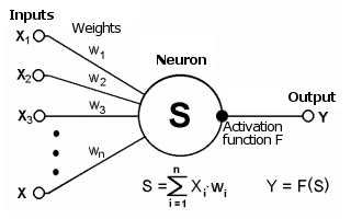
Schematic diagram of a neuron

This state is additionally processed using a non-linear activation function that generates the output value of a particular neuron. From the output, the signal will go further along the synapses of the next connected neurons (if any) or will become a component in the neural network's response (in case the current neuron is located in the last layer).

	(1)

	(2)

The presence of non-linearity enhances the computational capabilities of the network. We can use different activation functions, for example hyperbolic tangent or a logistic function (both of them are so-called S-shaped or sigmoid functions:

	(3)

As we will see below, MQL5 provides a large set of built-in activation functions. The choice of a function should be made based on the specific problem (regression, classification). Usually, it is possible to select several functions and then experimentally find the optimal one.

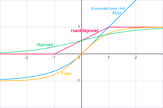
Popular activation functions

Activation functions can have different value ranges, limited or unlimited. In particular, the sigmoid (3) maps the data into the range [0,+1], which is better for classification problems, while the hyperbolic tangent maps data into the range [-1,+1], which is assumed better for regression and forecasting problems.

One of the important properties of the activation function is how its derivative is defined along the entire axis. The presence of a finite, nonzero derivative is critical for the backpropagation algorithm, which we will discuss later. S-shaped functions do satisfy this requirement. Moreover, the standard activation functions usually have a fairly simple analytical notation for the derivative, which guarantees their efficient computation. For example, for the sigmoid (3) we get:

	(4)

A single-layer neural network is shown in the following figure.

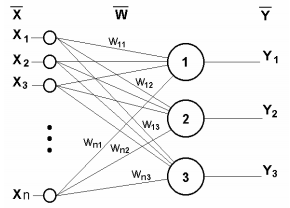
Single layer neural network

Its operating principle can be described mathematically by the following equation:

	(5)

Obviously, all the weight coefficients of one layer can fit into the W matrix, in which each wij element sets the value of the i-th connection of the j-th neuron. Thus, the process occurring in the neural network can be written in matrix form:

Y = F(X W)	(6)

where X and Y are the input and output signal vectors, respectively; F(V) is the activation function applied elementwise to the components of the vector V.

The number of layers and the number of neurons in each layer depends on the input data: their dimension, dataset size, distribution law, and many other factors. Often the network configuration is chosen by trial and error.

To illustrate this, I will show a diagram of a two-layer network.

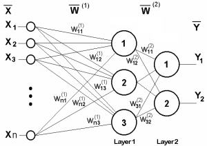
Two-layer neural network

Now consider one point which we have missed. From the figure of activation functions, it is obvious that there is some value of T, where S-shaped functions have a maximum slope and transmit signals well, while other functions have a characteristic breaking point (or several such points). Therefore, the main work of each neuron occurs near T. Usually T=0 or lies near 0, so it is desirable to have a capability to automatically shift the argument of the activation function to T.

This phenomenon was not reflected in formula (1), which should have looked like this:

	(7)

Such a shift is usually implemented by adding another pseudo-input to the neural layer. The value of this pseudo-input is always 1. Let's assign number 0 to this input. Then:

	(8)

where w0 = –T, x0 = 1.

In supervised learning algorithms, we have training data that has been previously prepared and marked by a human expert. In this data, the desired output vectors are associated with the input vectors.

The training process is implemented in the following stages.

1. Initialize weight matrix elements (usually small random values).

2. Input one of the vectors and compute the network reaction — this is the forward propagation of the signal; this phase will also be used during normal operation of a trained network.

3. Compute the difference between the ideal and the generated output values to find the network error, and then adjust the weights according to some formula depending on this error.

4. Continue in the loop from step 2 for all input vectors of the dataset until the error is reduced to the specified minimum level or below (successful completion of training) or until the predefined maximum number of training loops is reached (the neural network failed).

For a single-layer network, the weight adjustment formula is quite straightforward:

	(9)

	(10)

where δ is the network error (difference between the network response and the ideal), t and t+1 are the numbers of the current and next iteration; ν is the learning rate, 0<ν<1; i is the input index; j is the index of the neuron in the layer.

But what to in the case of a multi-layered network? This is where we come to the idea of backpropagation.

Backpropagation Algorithm

One of the best known neural network structures is the multilayer structure, in which each neuron of a particular layer is connected to all neurons of the previous layer or if it is the first layer, connected to all network inputs. Such neural networks are referred to as fully connected. Further explanation is provided for this structure. In many other types of neural networks, in particular, in convolutional networks, links connect limited areas of layers, the so-called cores, which somewhat complicates the addressing of network elements but does not affect the applicability of the backpropagation method.

Obviously, information about the error should be somehow passed from network outputs to its inputs, gradually leading through all layers taking into account the "conductivity" of the layers, i.e. the weights.

According to the least squares method, the objective function of the network error to be minimized is the following value:

	(11)

where yjpᴺ is the real output state of neuron j from the output layer N when the p-th image is input into it; djp is the ideal (desired) output state of this neuron.

The summation is implemented for all neurons of the output layer and over all processed images. The rate 1/2 is added only to get a nice derivative of E (twos are canceled), which will be used further for training (see equation (12)) and it is in any case weighted via an important parameter of the algorithm — the rate (which can be doubled or changed dynamically according to some conditions).

One of the most effective ways to minimize a function is based on the following: the best local directions to the extrema indicate the derivatives of this function at a particular point. A positive derivative leads to the maximum, and a negative derivative leads to the minimum. Of course, the maximum and minimum may turn out to be local, and additional tricks may be required to proceed to the global minimum, but we will leave this problem behind the scenes for now.

The described method is the Gradient Descent Method. According to it, the weights are adjusted based on the E derivative as follows:

	(12)

Here wij is the weight of the connection between the i-th neuron of layer n-1 and the j-th neuron of layer n,η is the learning rate.

Let us get back to the internal structure of the neuron and, on its basis, allocate each stage of calculations in the formula (12) into a partial derivative:

	(13)

As before, yj is the output of neuron j, while sj is the weighted sum of its input signals, i.e. the argument of the activation function. Since the factor dyj/dsj is the derivative of this function, this sets the requirement that the activation function should be differentiable on the entire x-axis for use in the considered backpropagation algorithm.

For example, in the case of hyperbolic tangent:

	(14)

The third factor in (13) ∂sj/∂wij is equal to neuron output yi of the previous layer (n-1). Why? In a multilayer network, the signal goes from the output of the previous layer neuron to the input of the current layer neuron. Therefore, formula (1) for sj can be rewritten in a more general way as follows:

	(15)

where M is the number of neurons in layer n-1, taking into account the neuron with a constant output state +1 which sets the offset; yi(n-1)=xij(n) is the i-th input of neuron j of layer n which is connected with the output of the i-th neuron of the (n-1)-th layer;

As for the first factor in (13), it is logical to expand it in error increments in the next higher layer (since the error values propagate in the opposite direction):

	(16)

Here summation for k is implemented among the neurons of layer n+1.

The first two factors in (13) for one layer (with neuron indices j) are repeated in (16) for the next layer (with indices k) as a coefficient before the weight wjk.

We introduce an intermediate variable which includes these two factors:

	(17)

As a result, we get a recursive formula for calculating the δj(n) of the layer n using the values δk(n+1) of the higher layer n+1.

	(18)

A new variable for the output layer, as before, is calculated based on the difference between the obtained and the desired result.

	(19)

Comparing with (9), here we have a derivative of the activation function. Note that in a network's output layer, depending on the task, the activation function may not be present.

Now we can write the expansion of formula (12) to adjust weights in the learning process:

	(20)

Sometimes, in order to give the weight adjustment process some inertia which smooths out sharp jumps in the derivative when moving over the surface of the objective function, formula (20) is supplemented with the weight change weight at the previous iteration:

	(21)

where µ is inertia coefficient and t is the number of the current iteration.

Thus, the complete neural network training algorithm using the backpropagation procedure is built as follows:

1. Initialize weight matrices with small random numbers.

2. Input one of the data vectors to the network and, in the normal operation mode, when the signals propagate from the inputs to the outputs, calculate the total NN result layer by layer according to the formulas for weighted summation (15) and activation f:

	(22)

Here, the neurons of the zero input layer are used only to feed input signals and do not have synapses and activation functions.

	(23)

Iq is the q-th component of the input vector fed into the zero layer.

3. If the network error is less than the specified small value, we stop the process as successful. If the error is significant, proceed to the next steps.

4. Compute for the output layer N: δ using the formula (19), as well as value changes Δw using formulas (20) or (21).

5. For all other layers in the reverse order, n=N-1,...1, compute δ and Δw using formulas (18) and (20) (or (18) and (21)), respectively.

6. Adjust all weights in the NN for iteration t based on the previous iteration t-1.

	(24)

7. Repeat the process in a loop starting from step 2.

The diagram of signals in the network being trained using the backpropagation algorithm is shown in the figure below.

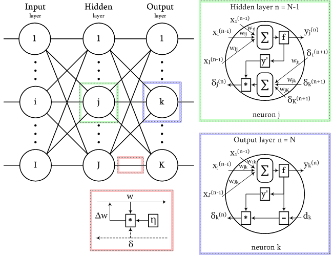
Signals in the backpropagation algorithm

All training images are alternately fed into the network so that it does not "forget" one as it memorizes others. Usually this is done in a random order, but because we locate the data in matrices and compute them as a single set, we will introduce another randomness element in our implementation which we will discuss a little later.

The use of matrices means that the weights of all layers, as well as the input and target training data, will be represented by matrices. Therefore, the above formulas, and accordingly, the algorithms will receive a matrix form. In other words, we cannot operate with separate vectors of input and raining data, while the entire loop from steps 2 to 7, will be calculated immediately for the entire dataset. One such loop is called a learning epoch.

Overview of activation functions

The article attachment contains the AF.mq5 script which displays on the chart thumbnails of all activation functions supported in MQL5 (in blue) and their derivatives (in red). The script automatically scales the thumbnails to fit all the functions into the window. If you need to get detailed images, I recommend maximizing the window. An example of an image generated by the script is shown below.

The correct choice of an activation function depends on the NN type and the problem. Moreover, several different activation functions can be used within one network. For example, SoftMax differs from other functions in that it processes the output values of the layer not elementwise, but in mutual connection: it normalizes them so that the values can be interpreted as probabilities (their sum is 1), which is used in the multiple classification.

This topic is very extensive, and it requires a separate article or a series of articles. For now, you should only note that all functions have both pros and cons, which can potentially lead to network failure. In particular, S-shaped functions are characterized by the 'vanishing gradient' problem, when the signals begin to fall on the S-curve's saturation sections and therefore the adjustment of the weights tends to zero). Monotonically increasing functions have the problem of explosive growth of the gradient ('exploding gradient', as the weights constantly increase causing the numerical overflow and NaN (Not A Number)). The more layers the network has, the more likely will be these two problems. There are various techniques to solve these problems, such as data normalization (both the input and the intermediate layers), network thinning algorithms ('dropout'), batch learning, noise and other regularization methods. We will consider some of them further.

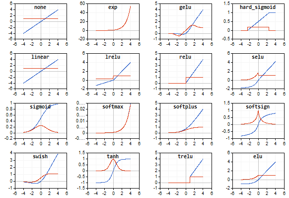
Demo script with all activation functions

Implementing a neural network in the MatrixNet class

Let us start writing a neural network class based on MQL5 matrices. The network consists of layers, so we will describe arrays of weights and output values of neurons for each layer. The number of layers will be stores in the n variable, while neuron weights and signals at each layer output will be stored in the 'weights' and 'outputs' matrices, respectively. Please note that 'outputs' refer to signals at any layer neuron outputs, not just at the network output. So, outputs[i] also describe the intermediate layers and even the zero layer to which the input data is written.

The indexing of 'weights' and 'outputs' arrays is shown in the following diagram (connections of each neuron with the +1 shift source are not shown for simplicity):

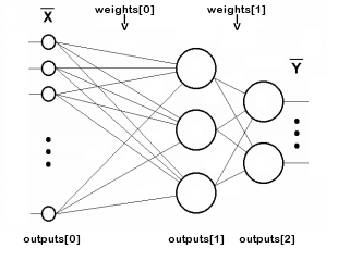
Indexing of matrix arrays in a two-layer network

The number n does not include the input layer since this layer does not require weights.

  class MatrixNet
  {
  protected:
     const int n;
     matrix weights[/* n */];
     matrix outputs[/* n + 1 */];
     ENUM_ACTIVATION_FUNCTION af;
     ENUM_ACTIVATION_FUNCTION of;
     double speed;
     bool ready;
     ...

Our network will support two types of activation functions (to be selected by the user): one for all layers except the output (stored in the 'af' variable), and a separate one for the output layer (stored in the 'of' variable). The 'speed' variable stores the learning rate (the η coefficient form the formula (20)).

The 'ready' variable contains an indication of a successful N object initialization.

The network constructor receives the integer array 'layers' which defines the number and sizes of all layers. The zero element sets the size of the input pseudo layer, i.e. the number of features in each input vector. The last element determines the size of the output layer, while all the rest define intermediate hidden layers. There must be at least two layers. The additional method 'allocate' has been written to allocate memory for matrix arrays (we will further develop it as the class expands).

  public:
     MatrixNet(const int &layers[], const ENUM_ACTIVATION_FUNCTION f1 = AF_TANH,
        const ENUM_ACTIVATION_FUNCTION f2 = AF_NONE):
        ready(false), af(f1), of(f2), n(ArraySize(layers) - 1)
     {
        if(n < 2) return;
        
        allocate();
        for(int i = 1; i <= n; ++i)
        {
           // NB: the weights matrix is transposed, i.e. indexes [row][column] specify [synapse][neuron]
           weights[i - 1].Init(layers[i - 1] + 1, layers[i]);
        }
        ...
     }
        
  protected:
     void allocate()
     {
        ArrayResize(weights, n);
        ArrayResize(outputs, n + 1);
        ...
     }

To initialize each weight matrix, the size of the previous layer layers[i - 1] is taken as the number of rows and one synapse is added to it for a constant adjustable shift source +1. As the number of columns, we use the size of the current layer layers[i]. In each weight matrix, the first index refers to the layer to the left of the matrix, while the second one refers to the one to the right.

Such numbering provides a simple record for the multiplication of signal vectors by layer matrices during forward propagation (normal network operation). During error backpropagation process (in training mode), it will be necessary to multiply the error vector of each higher layer by its transposed weight matrix in order to recalculate into errors for the lower layer.

In other words, since information inside the network moves in two opposite directions — working signals from inputs to outputs, and errors from outputs to inputs — weight matrices in one of these two directions should be used in the usual form, and in the second once they should be transposed. For the normal configuration, we use the matrix marking which facilitates the computation of the direct signal.

We will fill in the 'outputs' matrices along the process of the signal passing through the network. As for the weights, they should be randomly initialized. This is done by calling the 'randomize' method at the end of the constructor.

  public:
     MatrixNet(const int &layers[], const ENUM_ACTIVATION_FUNCTION f1 = AF_TANH,
        const ENUM_ACTIVATION_FUNCTION f2 = AF_NONE):
        ready(false), af(f1), of(f2), n(ArraySize(layers) - 1)
     {
        ...
        ready = true;
        randomize();
     }
     
     // NB: set values with appropriate distribution for specific activation functions
     void randomize(const double from = -0.5, const double to = +0.5)
     {
        if(!ready) return;
        
        for(int i = 0; i < n; ++i)
        {
           weights[i].Random(from, to);
        }
     }

The presence of the weight matrices is enough to implement the feed forward pass from the network input to the output. It is not a big problem that the weights have not yet been trained, as we will deal with training later.

     bool feedForward(const matrix &data)
     {
        if(!ready) return false;
        
        if(data.Cols() != weights[0].Rows() - 1)
        {
           PrintFormat("Column number in data %d <> Inputs layer size %d",
              data.Cols(), weights[0].Rows() - 1);
           return false;
        }
        
        outputs[0] = data; // input the data to the network
        for(int i = 0; i < n; ++i)
        {
           // expand each layer (except the last one) with one neuron for the bias signal
           // (there is no weight matrix to the right of the last layer, since the signal does not go further)
           if(!outputs[i].Resize(outputs[i].Rows(), weights[i].Rows()) ||
              !outputs[i].Col(vector::Ones(outputs[i].Rows()), weights[i].Rows() - 1))
              return false;
           // forward the signal from i-th layer to the (i+1)-th layer: weighted sum
           matrix temp = outputs[i].MatMul(weights[i]);
           // apply the activation function, the result is received into outputs[i + 1]
           if(!temp.Activation(outputs[i + 1], i < n - 1 ? af : of))
              return false;
        }
        
        return true;
     }

The number of columns in the input matrix data must match the number of rows in the zero weight matrix minus 1 (weight to bias signal).

To read the result of the regular network operation, use the getResults method. By default, it returns the output layer states matrix.

     matrix getResults(const int layer = -1) const
     {
        static const matrix empty = {};
        if(!ready) return empty;
        
        if(layer == -1) return outputs[n];
        if(layer < -1 || layer > n) return empty;
        
        return outputs[layer];
     }

We can evaluate the current quality of the model using the 'test' method, by feeding not only the input data matrix into it, but also the matrix with the desired network response.

     double test(const matrix &data, const matrix &target, const ENUM_LOSS_FUNCTION lf = LOSS_MSE)
     { 
        if(!ready || !feedForward(data)) return NaN();
        
        return outputs[n].Loss(target, lf);
     }

After the feed forward pass using the feedForward method, here we compute the "loss" of the given type. By default, this is the root mean square error (LOSS_MSE), which is suitable for regression and prediction problems. However, if the network is to be used for image classification, we should use a different type of scoring, such as LOSS_CCE cross entropy.

If a calculation error occurs, the method will return NaN (not a number).

Now let us proceed to the backpropagation. The backProp method also starts by checking whether the sizes of the target data and of the output layer match. The it calculates the derivative of the activation function for the output layer (if any) and the network "loss" at the output relative to the target data.

     bool backProp(const matrix &target)
     {
        if(!ready) return false;
     
        if(target.Rows() != outputs[n].Rows() ||
           target.Cols() != outputs[n].Cols())
           return false;
        
        // output layer
        matrix temp;
        if(!outputs[n].Derivative(temp, of))
           return false;
        matrix loss = (outputs[n] - target) * temp; // all data line by line

The loss matrix contains δ values from the formula (19).

Next, the following loop is executed for all layers except the output one:

        for(int i = n - 1; i >= 0; --i) // all layers except the output in reverse order
        {
           // remove pseudo-losses in the last element which we added as an offset source
           // since it is not a neuron and further error propagation is not applicable to it
           // (we do it in all layers except the last one where the shift element was not added)
           if(i < n - 1) loss.Resize(loss.Rows(), loss.Cols() - 1);
           
           matrix delta = speed * outputs[i].Transpose().MatMul(loss);

Here we see the exact formula (20): we get weight increments based on the learning rate η — δ of the current layer and the relevant outputs of the previous (lower) layer.

Next, for each layer, we calculate formula (18) to recursively obtain the rest δ values: we again use the derivative of the activation function and the multiplication of the higher δ to the transposed weight matrix. Index i in the outputs[] matrix corresponds to the layer with the weights in the (i-1)-th weights[] matrix, because the input pseudo-layer (outputs[0]) has no weights. In other words, in forward propagation, the weights[0] matrix is applied to outputs[0] and generates outputs[1]; weights[1] generates outputs[2], and so on. In contrast, in backpropagation, the indexes are the same: for example, outputs[2] (after differentiation) is multiplied by the transposed weights[2].

           if(!outputs[i].Derivative(temp, af))
              return false;
           loss = loss.MatMul(weights[i].Transpose()) * temp;

After computing 'loss' δ for the lower layer, we can adjust weights[i] matrix weight by correcting them for the earlier obtained delta.

           weights[i] -= delta;
        }
        return true;
     }

Now we are almost ready to implement a complete learning algorithm with a loop over epochs and feedForward and backProp method calls. However, we must first get back to some theoretical nuances which we have previously postponed.

Training and regularization

The NN is trained on the currently available training data. The network configuration (number of layers, number of neurons in layers, etc.), the learning rate and other characteristics are selected based on this data. Therefore, it is always possible to build a network powerful enough to produce any sufficiently small error on the training data. However, the ultimate purpose of using a neural network is to make it perform well on future unknown data (with the same implicit dependencies as in the training dataset).

The effect when a trained neural network performed too well on the training data but fails in the forward test is called overfitting. This effect should be avoided in every possible way. To avoid overfitting, we can use regularization. This implies the introduction of some additional conditions which evaluate the network's ability to generalize. There are many different ways to regularize, in particular:

• Analyzing the performance of the trained network on an additional validation dataset (different from the training one)
• Random discarding of a part of neurons or connections during training
• Network pruning after training
• Introducing noise into the input data
• Artificial data reproduction
• Weak constant decrease in the amplitude of weights during training
• Experimental selection of the volume and fine network configuration, when the network is still able to learn but does not overfit on the available data

We will implement some of them in our class.

First, we will enable the input of not only input and output training data ('data' and 'target' parameters, respectively) to the training method, but also of a validation dataset (it also consists of input and relevant output vectors: 'validation' and 'check').

As training progresses, the network error on the training data normally decreases quite monotonously (I used "normally" because if the learning rate or network capacity is incorrectly selected, the process can become unstable). However, if we calculate the network error on the validation set along this process, it will first decrease (while the network reveals the most important patterns in the data), and then it will start to grow as it overfits (when the network adapts to the particular features of the training dataset, but not the validation set). Thus, the learning process should be stopped when the validation error starts to rise. This is the "early stopping" approach.

In addition to two datasets, the 'train' method allows specifying the maximum number of training epochs, the desired accuracy (i.e. the average minimum error which is acceptable: in this case, training also stops with an indication of success) and the error calculation method (lf) .

The learning rate ('speed') is set equal to 'accuracy', but they can be set different to increase the flexibility of settings. This is because the rate will be adjusted automatically, and thus the initial approximate value is not so important.

     double train(const matrix &data, const matrix &target,
        const matrix &validation, const matrix &check,
        const int epochs = 1000, const double accuracy = 0.001,
        const ENUM_LOSS_FUNCTION lf = LOSS_MSE)
     {
        if(!ready) return NaN();
        
        speed = accuracy;
        ...

We will save the current epoch network error values in the variables mse and msev, for the training and validation sets. To exclude the response to inevitable random fluctuations, we will need to average the errors over a certain period p, which is calculated from the total given number of epochs. The smoothed error values will be stored in the msema and msevma variables, and their previous values will be saved in the msemap and msevmap variables.

        double mse = DBL_MAX;
        double msev = DBL_MAX;
        double msema = 0;       // MSE averaging of the training set
        double msemap = 0;      // MSE averaging of the training set in the previous epoch
        double msevma = 0;      // MSE averaging of the validation dataset
        double msevmap = 0;     // MSE averaging of the validation dataset in the previous epoch
        double ema = 0;         // exponential smoothing factor
        int p = 0;              // EMA period
        
        p = (int)sqrt(epochs);  // empirically choose the period of the EMA averaging of errors
        ema = 2.0 / (p + 1);
        PrintFormat("EMA for early stopping: %d (%f)", p, ema);

Next, we run a loop of training epochs. We allow not to provide validation data, since later we will implement another regularization method, Dropout. If the validation dataset is not empty, we calculate msev by calling the 'test' method for this set. In any case, we calculate mse by calling 'test' for the training set. The 'test' calls the feedForward method and calculates the error of the network result relative to the target values.

        int ep = 0;
        for(; ep < epochs; ep++)
        {
           if(validation.Rows() && check.Rows())
           {
              // if there is validation, run it before normal pass/training
              msev = test(validation, check, lf);
              // smooth errors
              msevma = (msevma ? msevma : msev) * (1 - ema) + ema * msev;
           }
           mse = test(data, target, lf);  // enable feedForward(data) run
           msema = (msema ? msema : mse) * (1 - ema) + ema * mse;
           ...

First, we check that the error value is a valid number. Otherwise, the network has overflowed, or incorrect data has been input.

           if(!MathIsValidNumber(mse))
           {
              PrintFormat("NaN at epoch %d", ep);
              break; // will return NaN as error indication
           }

If the new error has become larger than the previous one with some "tolerance", which is determined from the ratio of the sizes of the training and validation datasets, the loop is interrupted.

           const int scale = (int)(data.Rows() / (validation.Rows() + 1)) + 1;
           if(msevmap != 0 && ep > p && msevma > msevmap + scale * (msemap - msema))
           {
              // skip the first p epochs to accumulate values for averaging
              PrintFormat("Stop by validation at %d, v: %f > %f, t: %f vs %f", ep, msevma, msevmap, msema, msemap);
              break;
           }
           msevmap = msevma;
           msemap = msema;
           ...

If the error continues to decrease or it does not grow, save new error values to compare with the next epoch result.

If the error has reached the required accuracy, the training is considered to be completed and thus we exit the loop.

           if(mse <= accuracy)
           {
              PrintFormat("Done by accuracy limit %f at epoch %d", accuracy, ep);
              break;
           }

In addition, the virtual method 'progress' is called in the loop, which can be overridden in derived classes of the network. It can be used to interrupt training in response to some user actions. The standard implementation of 'progress' will be shown later.

           if(!progress(ep, epochs, mse, msev, msema, msevma))
           {
              PrintFormat("Interrupted by user at epoch %d", ep);
              break;
           }

Finally, if the loop was not interrupted by any of the above conditions, we start the error backpropagation process using backProp.

           if(!backProp(target))
           {
              mse = NaN(); // error flag
              break;
           }
        }
        
        if(ep == epochs)
        {
           PrintFormat("Done by epoch limit %d with accuracy %f", ep, mse);
        }
        
        return mse;
     }

The default 'progress' method logs learning metrics once per second.

     virtual bool progress(const int epoch, const int total,
        const double error, const double valid = DBL_MAX,
        const double ma = DBL_MAX, const double mav = DBL_MAX)
     {
        static uint trap;
        if(GetTickCount() > trap)
        {
           PrintFormat("Epoch %d of %d, loss %.5f%s%s%s", epoch, total, error,
              ma == DBL_MAX ? "" : StringFormat(" ma(%.5f)", ma),
              valid == DBL_MAX ? "" : StringFormat(", validation %.5f", valid),
              valid == DBL_MAX ? "" : StringFormat(" v.ma(%.5f)", mav));
           trap = GetTickCount() + 1000;
        }
        return !IsStopped();
     }

If 'true' is returned, training continues, while 'false' will cause the loop to break.

In addition to the "early termination", the MatrixNet class can randomly disable some of the connections similar to dropout.

According to the traditional dropout method, randomly selected neurons are temporarily excluded from the network. However, implementing this would be costly, since the algorithm uses matrix operations. To exclude neurons from the layer, we would need to reformat the weight matrices at each iteration and partially copy them. It is much easier and more efficient to set random weights to 0, which will break connections. Of course, at the beginning of each epoch, the program must restore temporarily disabled weights to their previous state, and then randomly select new ones to disable in the next epoch.

The number of temporarily reset connections is set using the enableDropOut method as a percentage of the total number of network weights. By default, the dropOutRate variable is 0, so the mode is disabled.

     void enableDropOut(const uint percent = 10)
     {
        dropOutRate = (int)percent;
     }

The dropout principle is to save the current state of the weight matrices in some additional storage (it is implemented by the DropOutState class) and to reset randomly selected network connections. After training the network in the resulting modified form for one epoch, the reset matrix elements are restored from the storage, and the procedure is repeated: other random weights are selected and reset, the network is trained with them, and so on. I suggest that you explore how the DropOutState works on your own.

Adaptive Learning Rate

So far, it has been assumed that we are using a constant learning rate (the 'speed' variable), but this is not practical (learning can be very slow at low speeds, or "overexcited" at high rates).

One of the learning rate adjustment forms is used in a special modification of the backpropagation algorithm. It is called "rprop" (Resilient Propagation). The algorithm checks for each weight whether the sign of the delta increments at the previous and current iteration is the same. If the signs are the same, the direction of the gradient is preserved, and in this case the speed can be increased selectively for the given weight. For those weights where the sign of the gradient has changed, it can be better to slow down.

Since matrices calculate all the data at once at each epoch, the value and sign of the gradient for each weight accumulate (and average) the behavior of the entire dataset. Therefore, the technology is more accurately referred to as "batch rprop".

All lines of code in the MatrixNet class that implement this enhancement are provided with the BATCH_PROP macros. Before including the header file MatrixNet.mqh into your source code, it is recommended to enable adaptive rate using the following directive:

  #define BATCH_PROP

Pay attention that instead of the 'speed' variable this mode uses an array of 'speed' matrices. We also need to store weight increments from the last epoch in an array of 'deltas' matrices.

  class MatrixNet
  {
  protected:
     ...
     #ifdef BATCH_PROP
     matrix speed[];
     matrix deltas[];
     #else
     double speed;
     #endif

The acceleration and deceleration coefficients, as well as the maximum and minimum speeds, are set in 4 additional variables.

     double plus;
     double minus;
     double max;
     double min;

We allocate memory for the new arrays and set default variable values in the already familiar 'allocate' method.

     void allocate()
     {
        ArrayResize(weights, n);
        ArrayResize(outputs, n + 1);
        ArrayResize(bestWeights, n);
        dropOutRate = 0;
        #ifdef BATCH_PROP
        ArrayResize(speed, n);
        ArrayResize(deltas, n);
        plus = 1.1;
        minus = 0.1;
        max = 50;
        min = 0.0;
        #endif
     }

To set other values for these variables before we begin training, use the setupSpeedAdjustment method.

In the MatrixNet constructor, we initialize 'speed' and 'deltas' matrices by copying the array of 'weight' matrices — this is a more convenient way to get matrices of same sizes along the network layers. Then, 'speed' and 'deltas' are filled with meaningful data in next steps. At the beginning of the 'train' method, instead of simply assigning the accuracy in the scalar variable 'speed', this value is used to fill all matrices in the 'speed' array.

     double train(const matrix &data, const matrix &target,
        const matrix &validation, const matrix &check,
        const int epochs = 1000, const double accuracy = 0.001,
        const ENUM_LOSS_FUNCTION lf = LOSS_MSE)
     {
        ...
        #ifdef BATCH_PROP
        for(int i = 0; i < n; ++i)
        {
           speed[i].Fill(accuracy); // adjust speeds on the fly
           deltas[i].Fill(0);
        }
        #else
        speed = accuracy;
        #endif
        ...
     }

Inside the backProp method, the increment expression now refers to the corresponding layer's matrix rather than a scalar. Immediately after receiving the 'delta' increments, we call the adjustSpeed method (shown below), passing to it the product of 'delta * deltas[i]' to compare the previous and new directions. Finally, we save the new weight increments into 'deltas[i]' to analyze them at the next epoch.

     bool backProp(const matrix &target)
     {
        ...
        for(int i = n - 1; i >= 0; --i) // all layers except the output in reverse order
        {
           ...
           #ifdef BATCH_PROP
           matrix delta = speed[i] * outputs[i].Transpose().MatMul(loss);
           adjustSpeed(speed[i], delta * deltas[i]);
           deltas[i] = delta;
           #else
           matrix delta = speed * outputs[i].Transpose().MatMul(loss);
           #endif
           ...
        }
        ...
     }

The adjustSpeed method is quite simple. A positive sign in the matrix product element indicates that the gradient is preserved, and the speed increases by 'plus' times, but no more than 'max' value. A negative sign indicates a change in the gradient, and the speed decreases by 'minus' times, but it cannot be less than 'min'.

     void adjustSpeed(matrix &subject, const matrix &product)
     {
        for(int i = 0; i < (int)product.Rows(); ++i)
        {
           for(int j = 0; j < (int)product.Cols(); ++j)
           {
              if(product[i][j] > 0)
              {
                 subject[i][j] *= plus;
                 if(subject[i][j] > max) subject[i][j] = max;
              }
              else if(product[i][j] < 0)
              {
                 subject[i][j] *= minus;
                 if(subject[i][j] < min) subject[i][j] = min;
              }
           }
        }
     }

Saving and Restoring the Best State of the Trained Network

So, the network is trained in loop, in iterations called 'epochs': in each epoch, all vectors of the training dataset pass through the network, being placed in a matrix, in which records are arranged in rows and their signs are in columns. For example, each record can store a quote bar, while columns can store OHLC prices and volumes.

Although the weight adjusting process is performed along a gradient, it is random in the sense that due to the unevenness of the objective function of the problem being solved and the variable speed, we can periodically get to "bad" settings before finding a new minimum of the network error. We have no guarantee that an increase in the epoch number comes with a certain improvement of the quality of the trained model and with the reduction of the network error.

In this regard, it makes sense to constantly monitor the overall error of the network: if after the current epoch the error updates the minimum, the found weights should be remembered. For these purposes, we will use another array of weight matrices and the 'Stats' structure with learning metrics.

  class MatrixNet
  {
     ...
  public:
     struct Stats
     {
        double bestLoss; // smallest error for all epochs
        int bestEpoch;   // index of the epoch with the minimum error
        int epochsDone;  // total number of completed epochs
     };
     
     Stats getStats() const
     {
        return stats;
     }
     
  protected:
     matrix bestWeights[];
     Stats stats;
     ...

Inside the train method, before starting the loop over epochs, we initialize the structure with statistics.

     double train(const matrix &data, const matrix &target,
        const matrix &validation, const matrix &check,
        const int epochs = 1000, const double accuracy = 0.001,
        const ENUM_LOSS_FUNCTION lf = LOSS_MSE)
     {
        ...
        stats.bestLoss = DBL_MAX;
        stats.bestEpoch = -1;
        DropOutState state(dropOutRate);

Inside the loop, if an error value less than the minimum known value is found, we save all weight matrices in bestWeights.

        int ep = 0;
        for(; ep < epochs; ep++)
        {
           ...
           const double candidate = (msev != DBL_MAX) ? msev : mse;
           if(candidate < stats.bestLoss)
           {
              stats.bestLoss = candidate;
              stats.bestEpoch = ep;
              // save best weights from 'weights'
              for(int i = 0; i < n; ++i)
              {
                 bestWeights[i].Assign(weights[i]);
              }
           }
        }
        ...

After training, it is easy to query both the final network weights and the best weights.

     bool getWeights(matrix &array[]) const
     {
        if(!ready) return false;
        
        ArrayResize(array, n);
        for(int i = 0; i < n; ++i)
        {
           array[i] = weights[i];
        }
        
        return true;
     }
     
     bool getBestWeights(matrix &array[]) const
     {
        if(!ready) return false;
        if(!n || !bestWeights[0].Rows()) return false;
        
        ArrayResize(array, n);
        for(int i = 0; i < n; ++i)
        {
           array[i] = bestWeights[i];
        }
        
        return true;
     }

These arrays of matrices can be saved to a file so that later we can restore an already trained and ready-to-work network. This is done in a separate constructor.

     MatrixNet(const matrix &w[], const ENUM_ACTIVATION_FUNCTION f1 = AF_TANH,
        const ENUM_ACTIVATION_FUNCTION f2 = AF_NONE):
        ready(false), af(f1), of(f2), n(ArraySize(w))
     {
        if(n < 2) return;
        
        allocate();
        for(int i = 0; i < n; ++i)
        {
           weights[i] = w[i];
           #ifdef BATCH_PROP
           speed[i] = weights[i];  // instead .Init(.Rows(), .Cols())
           deltas[i] = weights[i]; // instead .Init(.Rows(), .Cols())
           #endif
        }
        
        ready = true;
     }

Later, we will see a practical example, showing how to save and read ready-made networks.

Visualization of Network Training Progress

The result of the 'progress' method which outputs periodic logs is not very clear. Therefore, the MatrixNet.mqh file also implements the MatrixNetVisual class derived from MatrixNet, which displays a graph with changing training errors by epochs.

Graphic display is provided by the standard CGraphic class (available in MetaTrader 5), or rather, a small CMyGraphic class derived from it.

The object of this class is part of MatrixNetVisual. Also, inside the "visualized" network we have an array of 5 curves and arrays of the double type, intended for the displayed lines.

  class MatrixNetVisual: public MatrixNet
  {
     CMyGraphic graphic;
     CCurve *c[5];
     double p[], x[], y[], z[], q[], b[];
     ...

where:

p is the epoch number (common horizontal X axis for all curves);

x is the training dataset error (Y)

y is the validation dataset error (Y)

z is the smoothed validation error (Y)

q is the smoothed learning error (Y)

b is the point (epoch) with the minimum error (Y)

The 'graph' method called from the MatrixNetVisual constructor creates a graphical object the size of the entire window. The five curves (CCurve) described above are also added here.

   void graph()
   {
      ulong width = ChartGetInteger(0, CHART_WIDTH_IN_PIXELS);
      ulong height = ChartGetInteger(0, CHART_HEIGHT_IN_PIXELS);

      bool res = false;
      const string objname = "BPNNERROR";
      if(ObjectFind(0, objname) >= 0) res = graphic.Attach(0, objname);
      else res = graphic.Create(0, objname, 0, 0, 0, (int)(width - 0), (int)(height - 0));
      if(!res) return;

      c[0] = graphic.CurveAdd(p, x, CURVE_LINES, "Training");
      c[1] = graphic.CurveAdd(p, y, CURVE_LINES, "Validation");
      c[2] = graphic.CurveAdd(p, z, CURVE_LINES, "Val.EMA");
      c[3] = graphic.CurveAdd(p, q, CURVE_LINES, "Train.EMA");
      c[4] = graphic.CurveAdd(p, b, CURVE_POINTS, "Best/Minimum");
      ...
   }

public:
   MatrixNetVisual(const int &layers[], const ENUM_ACTIVATION_FUNCTION f1 = AF_TANH,
      const ENUM_ACTIVATION_FUNCTION f2 = AF_NONE): MatrixNet(layers, f1, f2)
   {
      graph();
   }

In the overridden 'progress' method, the arguments are added to the appropriate double arrays, and then the 'plot' method is called to update the image.

     virtual bool progress(const int epoch, const int total,
        const double error, const double valid = DBL_MAX,
        const double ma = DBL_MAX, const double mav = DBL_MAX) override
     {
        // fill all the arrays
        PUSH(p, epoch);
        PUSH(x, error);
        if(valid != DBL_MAX) PUSH(y, valid); else PUSH(y, nan);
        if(ma != DBL_MAX) PUSH(q, ma); else PUSH(q, nan);
        if(mav != DBL_MAX) PUSH(z, mav); else PUSH(z, nan);
        plot();
        
        return MatrixNet::progress(epoch, total, error, valid, ma, mav);
     }

The 'plot' method completes and plots of the curves.

   void plot()
   {
      c[0].Update(p, x);
      c[1].Update(p, y);
      c[2].Update(p, z);
      c[3].Update(p, q);
      double point[1] = {stats.bestEpoch};
      b[0] = stats.bestLoss;
      c[4].Update(point, b);
      ...
      graphic.CurvePlotAll();
      graphic.Update();
   }

You can explore further technical details of the visualization process on your own. We will soon see how it looks like on the screen.

Test Script

MatrixNet family classes are ready for the first test. It will be the MatrixNet.mq5 script, in which the initial data is artificially generated based on a known analytical record. We will use the formula from the Machine Learning help topic, which provides a native backpropagation training example that is not as versatile as our classes and therefore requires significant coding (compare the number of rows with and without using the class below).

f = ((x + y + z)^2 / (x^2 + y^2 + z^2)) / 3

The only small difference in our formula is that the value is divided by 3, which gives the function a range of 0 to 1.

The form of the function can be evaluated using the following figure, where the surfaces (x<->y) are shown for three different z values: 0.05, 0.5 and 5.0.

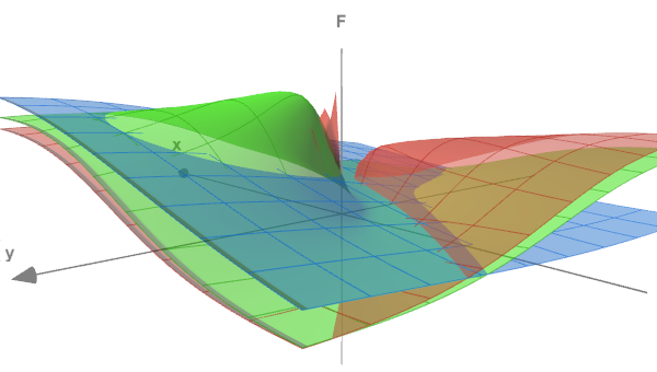
Test function in 3 sections

In the script input variables, we will specify the number of training epochs, the accuracy (terminal error) and the noise intensity, which we can optionally add to the generated data (this will bring the experiment closer to real problems and will demonstrate how the noise makes it difficult to identify dependencies). RandomNoise is 0 by default, and thus there is no noise.

  input int Epochs = 1000;
  input double Accuracy = 0.001;
  input double RandomNoise = 0.0;

The experimental data is generated by the CreateData function. Its matrix parameters 'data' and 'target' will be filled with the points of the function described above. The number of points is 'count'. One input vector (row of the 'data' matrix) has 3 columns (for x, y, z). The output vector (row of the 'target' matrix) is the single value of f. Points (x,y,z) are randomly generated in the range from -10 to +10.

  bool CreateData(matrix &data, matrix &target, const int count)
  { 
     if(!data.Init(count, 3) || !target.Init(count, 1))
        return false;
     data.Random(-10, 10);
     vector X1 = MathPow(data.Col(0) + data.Col(1) + data.Col(2), 2);
     vector X2 = MathPow(data.Col(0), 2) + MathPow(data.Col(1), 2) + MathPow(data.Col(2), 2);
     if(!target.Col(X1 / X2 / 3.0, 0))
        return false;
     if(RandomNoise > 0)
     {
        matrix noise;
        noise.Init(count, 3);
        noise.Random(0, RandomNoise);
        data += noise - RandomNoise / 2;
        
        noise.Resize(count, 1);
        noise.Random(-RandomNoise / 2, RandomNoise / 2);
        target += noise;
     }
     return true; 
  }

The noise intensity in RandomNoise is set as the amplitude of the additional spread of the correct coordinates and the function value obtained for them. Given that the function maximum value is 1.0, this level of noise will make it almost unrecognizable.

To use the neural network, we include the MatrixNet.mqh header file and define the BATCH_PROP macro before this preprocessor directive to enable accelerated learning at a variable rate.

  #define BATCH_PROP
  #include <MatrixNet.mqh>

In the main script function, we define the network configuration (the number of layers and their sizes) using the 'layers' array, which we pass to the MatrixNetVisual constructor. Training and validation datasets are generated by calling CreateData twice.

  void OnStart()
  {
     const int layers[] = {3, 11, 7, 1};
     MatrixNetVisual net(layers);
     matrix data, target;
     CreateData(data, target, 100);
     matrix valid, test;
     CreateData(valid, test, 25);
     ...

In practice, we should normalize the source data, remove the outliers, check the factors for independence before sending them to the network. But in this case we generate the data ourselves.

The model is trained using the 'train' method on the 'data' and 'target' matrices. An early termination will occur as performance deteriorates on the valid/test set, but on non-noisy data, we are likely to reach the required accuracy or max loops, whichever happens faster.

     Print("Training result: ", net.train(data, target, valid, test, Epochs, Accuracy));
     matrix w[];
     if(net.getBestWeights(w))
     {
        MatrixNet net2(w);
        if(net2.isReady())
        {
           Print("Best copy on training data: ", net2.test(data, target));
           Print("Best copy on validation data: ", net2.test(valid, test));
        }
     }

After training, we request the matrices of the best found weights and, to check, construct another network instance based on them, the net2 object. After that run the network on both datasets and print their error values in the log.

Since the script uses a network with learning progress visualization, we start a loop waiting for the user's command to complete the script so that the user can study the graph.

     while(!IsStopped())
     {
        Sleep(1000);
     }
  }

When running the script with default parameters, we can get something like in the following figure (each run will be different from the others due to random data generation and network initialization).

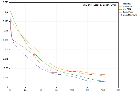
Network error dynamics during training

Errors on the training and validation sets are shown as blue and red lines, respectively, and their smoothed versions are green and yellow. We can clearly see that as training progresses, all types of errors decrease, but after a certain moment, the validation error becomes larger than the error of the training set. Near the right edge of the graph its increase is noticeable, resulting in an "early termination". The best network configuration is circled.

The journal can be as follows:

  EMA for early stopping: 31 (0.062500)
  Epoch 0 of 1000, loss 0.20296 ma(0.20296), validation 0.18167 v.ma(0.18167)
  Epoch 120 of 1000, loss 0.02319 ma(0.02458), validation 0.04566 v.ma(0.04478)
  Stop by validation at 155, v: 0.034642 > 0.034371, t: 0.016614 vs 0.016674
  Training result: 0.015707719706513287
  Best copy on training data: 0.015461956812387292
  Best copy on validation data: 0.03211748853774414

If we start adding noise to the data using the RandomNoise parameter, the learning rate will noticeably decrease, and if there is too much noise, the error of the trained network will increase, or it will stop learning altogether.

For example, here is what the graph with the noise 3.0 looks like.

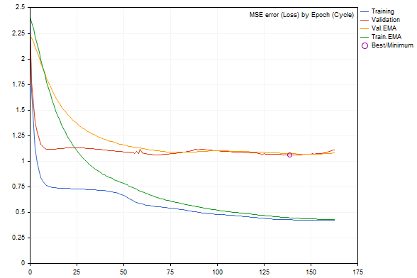
Network error dynamics in training with added noise

According to the log, the error value is much worse.

  Epoch 0 of 1000, loss 2.40352 ma(2.40352), validation 2.23536 v.ma(2.23536)
  Stop by validation at 163, v: 1.082419 > 1.080340, t: 0.432023 vs 0.432526
  Training result: 0.4244786772678285
  Best copy on training data: 0.4300476339855798
  Best copy on validation data: 1.062895214094978

So, the neural network toolkit works well. Now, let's move on to more practical examples: an indicator and an Expert Advisor.

Predictive Indicator

As an example of a NN-based predictive indicator, let us consider BPNNMatrixPredictorDemo.mq5, which is a modification of an existing indicator from the CodeBase. The NN is implemented in MQL5, without the use of matrices, by porting an earlier version of the same indicator from C++ (with detailed description, including relevant parts of NN theory).

The indicator operates by forming input vectors of a given length from past increments of the EMA-averaged price on intervals between bars spaced from each other by the Fibonacci sequence (1,2,3,5,8,13,21,34,55,89,144. ..). Based on this information, the indicator should predict the price increment on the next bar (to the right of the historical bars included in the corresponding vector). The size of the vector is determined by the user-specified size of the NN input layer (_numInputs). The number of layers (up to 6) and their sizes are specified in other input variables.

  input int _lastBar = 0;     // Last bar in the past data
  input int _futBars = 10;    // # of future bars to predict
  input int _smoothPer = 6;   // Smoothing period
  input int _numLayers = 3;   // # of layers including input, hidden & output (2..6)
  input int _numInputs = 12;  // # of inputs (that is neurons in input 0-th layer)
  input int _numNeurons1 = 5; // # of neurons in the 1-st hidden or output layer
  input int _numNeurons2 = 1; // # of neurons in the 2-nd hidden or output layer
  input int _numNeurons3 = 0; // # of neurons in the 3-rd hidden or output layer
  input int _numNeurons4 = 0; // # of neurons in the 4-th hidden or output layer
  input int _numNeurons5 = 0; // # of neurons in the 5-th hidden or output layer
  input int _ntr = 500;       // # of training sets / bars
  input int _nep = 1000;      // Max # of epochs
  input int _maxMSEpwr = -7;  // Error (as power of 10) for training to stop; mse < 10^this

Also, we indicate here the maximum size of the training dataset (_ntr), the maximum number of epochs (_nep) and the minimum MSE error (_maxMSEpwr).

The price EMA averaging period is specified in _smoothPer.

By default, the indicator takes training data starting from the last bar (_lastBar is equal to 0) and makes a forecast for _futBars ahead (obviously, having a forecast for 1 bar at the network output, we can gradually "push" it into the input vector to predict several subsequent bars). If a positive number is specified in _lastBar, we will get a forecast as of the corresponding number of bars in the past, which will allow us to visually evaluate it by comparing it with the existing quotes.

The indicator outputs 3 buffers:

• light green line with the target values of the training dataset
• blue line with the network output on the training dataset
• red line for the forecast

The application part of the indicator generating datasets and visualizing the results (both initial data and forecast) has not changed.

The main modifications have been made in two functions Train and Test: now they completely delegate the NN work to the objects of the MatrixNet class. The 'Train' function trains the network based on the collected data and returns an array with the network weights (when running in the tester, training is done only once, and when running online, opening a new bar causes repeated training; this can be changed in the source code). The 'Test' function recreates the network by weights and performs a regular one-time prediction calculation. It would be more optimal to save the object of the trained network and exploit it without recreating it. We will do this in the next example, with the EA. As for the indicator, I deliberately use the original code structure of the old version to make it more convenient to compare coding approaches with and without matrices. In particular, you can pay attention to the fact that in the matrix version we do not have to run the vectors through the network in a loop one at a time and manually reshape the data arrays in accordance with their dimension.

Below is the indicator with default settings on the EURUSD, H1 chart.

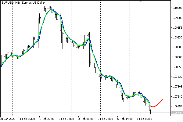
Prediction made by a neural network based indicator

Please note that the indicator is presented here to demonstrate the performance of a neural network. It is not recommended for use for making trading decisions in its current simplified form.

Storing NNs in Files

The source data incoming from the market can change rapidly, and some traders find it worthwhile to train the network on-the-fly (every day, every session, etc.) on the most recent datasets. However, it can be costly, and not so relevant for medium- and long-term trading systems which operate based in day data. In such cases, it is desirable to save the trained network so that later it can be quickly loaded and used.

For this purpose, within the framework of this article, we have created the MatrixNetStore class which is defined in the MatrixNetStore.mqh header file. The class includes template methods 'save' and 'load' which expect any class from the MatrixNet family as the M template parameter (now we have only two classes, including MatrixNetVisual, but you can expand the set if you wish). Both methods have an argument with a file name and operate with standard NN data: the number of layers, their size, weight matrices, and activation functions.

Here is how the network is saved.

  class MatrixNetStore
  {
     static string signature;
  public:
     template<typename M> // M is a MatrixNet
     static bool save(const string filename, const M &net, Storage *storage = NULL, const int flags = 0)
     {
        // get the matrix of weights (the best weights, if any)
        matrix w[];
        if(!net.getBestWeights(w))
        {
           if(!net.getWeights(w))
           {
              return false;
           }
        }
        // open file
        int h = FileOpen(filename, FILE_WRITE | FILE_BIN | FILE_SHARE_READ | FILE_SHARE_WRITE | FILE_ANSI | flags);
        if(h == INVALID_HANDLE) return false;
        // write network metadata
        FileWriteString(h, signature);
        FileWriteInteger(h, net.getActivationFunction());
        FileWriteInteger(h, net.getActivationFunction(true));
        FileWriteInteger(h, ArraySize(w));
        // write weight matrices
        for(int i = 0; i < ArraySize(w); ++i)
        {
           matrix m = w[i];
           FileWriteInteger(h, (int)m.Rows());
           FileWriteInteger(h, (int)m.Cols());
           double a[];
           m.Swap(a);
           FileWriteArray(h, a);
        }
        // if user data is provided, write it
        if(storage)
        {
          if(!storage.store(h)) Print("External info wasn't saved");
        }
        
        FileClose(h);
        return true;
     }
     ...
  };
     
  static string MatrixNetStore::signature = "BPNNMS/1.0";

Pay attention to the following points. A signature is written at the beginning of the file so that it can be used to check the correctness of the file format (the signature can be changed: the class provides methods for this). In addition, the 'save' method allows, if necessary, to add any user data to the standard information about the network: you should simply pass a pointer to an object of the special Storage interface.

  class Storage
  {
  public:
     virtual bool store(const int h) = 0;
     virtual bool restore(const int h) = 0;
  };

A network can be restored from the file accordingly.

  class MatrixNetStore
  {
     ...
     template<typename M> // M is a MatrixNet
     static M *load(const string filename, Storage *storage = NULL, const int flags = 0)
     {
        int h = FileOpen(filename, FILE_READ | FILE_BIN | FILE_SHARE_READ | FILE_SHARE_WRITE | FILE_ANSI | flags);
        if(h == INVALID_HANDLE) return NULL;
        // check the format by signature
        const string header = FileReadString(h, StringLen(signature));
        if(header != signature)
        {
           FileClose(h);
           Print("Incorrect file header");
           return NULL;
        }
        // read standard network metadata set
        const ENUM_ACTIVATION_FUNCTION f1 = (ENUM_ACTIVATION_FUNCTION)FileReadInteger(h);
        const ENUM_ACTIVATION_FUNCTION f2 = (ENUM_ACTIVATION_FUNCTION)FileReadInteger(h);
        const int size = FileReadInteger(h);
        matrix w[];
        ArrayResize(w, size);
        // read weight matrices
        for(int i = 0; i < size; ++i)
        {
           const int rows = FileReadInteger(h);
           const int cols = FileReadInteger(h);
           double a[];
           FileReadArray(h, a, 0, rows * cols);
           w[i].Swap(a);
           w[i].Reshape(rows, cols);
        }
        // read user data
        if(storage)
        {
           if(!storage.restore(h)) Print("External info wasn't read");
        }
        // create a network object
        M *m = new M(w, f1, f2);
        
        FileClose(h);
        return m;
     }

Now we are ready to proceed to the final example in this article, to a trading robot.

Predictive Expert Advisor

As a strategy for the TradeNN.mq5 predictive EA, we will use a fairly simple principle: trade in the predicted direction of the next bar. Our purpose is to demonstrate neural network technologies in action, but not to explore all foreseeable applicability factors in the context of profitability.

The initial data will be price increments on a given number of bars. Optionally, it will be possible to analyze not only the current symbol, but also additional ones, which theoretically will allow us to identify interdependencies (for example, if one ticker indirectly "follows" another or their combinations). The only output of the network will not be interpreted as a target price. Instead, in order to simplify the system, we will analyze the sign: positive - buy, negative - sell.

In other words, the network operation scheme is in a sense hybrid: on the one hand, the network will solve the regression problem, but on the other hand, we will select a trading action from two, as in classification. In the future, it will be possible to increase the number of neurons in the output layer up to the number of trading situations and to apply the SoftMax activation function. However, in order to train such a network, it will be necessary to label quotes automatically or manually according to the situations.

The strategy is deliberately made very simple in order to focus on network parameters, not the strategy.

A comma separated list of instruments to be analyzed is specified in the 'Symbols' input parameter. The symbol of the current chart should go first; it is on the traded symbol.

  input string Symbols = "XAGUSD,XAUUSD,EURUSD";
  input int Depth = 5; // Vector size (bars)
  input int Reserve = 250; // Training set size (vectors)

I have chosen these symbols as default because silver and gold are considered correlated assets, and there is relatively little high-impact news (compared to currencies), so, we can try to analyze both silver against gold (as it is now) and gold against silver. As for EURUSD, this pair is added as the basis of the entire market. The presence of news is not important, since it works as a predictor, not a predictive variable.

Among the other most important parameters is the number of bars (Depth) for each instrument that form the vector. For example, if Symbols is set to 3 tickers and Depth is set to 5 (default), then the total size of the network's input vector is 15.

The Reserve parameter allows setting the sample length (the number of vectors that are formed from the nearest quotes history). The default value is 250 because our test will use the daily time frame, and 250 is approximately 1 year. Accordingly, Depth equal to 5 is a week.

Of course, you can change any settings, including the timeframe, but on higher timeframes, like D1, fundamental patterns are supposedly more pronounced than spontaneous market reactions to momentary circumstances.

Please also note that when launched in the tester, it approximately pre-loads 1 year of quotes, so increasing the amount of requested training data on D1+ will require skipping a certain number of initial bars, waiting for a sufficient number of them to accumulate.

Similar to the previous examples, we should specify the number of training epochs and accuracy (which is also the initial speed, then the speed will be dynamically selected for each synapse by "rprop") in the parameters.

  input int Epochs = 1000;
  input double Accuracy = 0.0001; // Accuracy (and training speed)

In this Expert Advisor, the NN will have 5 layers: one input, 3 hidden and one output. The size of the input layer determines the input vector, and the second and third layers are selected with HiddenLayerFactor. For the penultimate layer, we will use an empirical formula (see the source code below) to have its size between the preceding and the output one (single).

  input double HiddenLayerFactor = 2.0; // Hidden Layers Factor (to vector size)
  input int DropOutPercentage = 0; // DropOut Percentage

We will also use this example to test the dropout regularization method: the percentage of randomly reset weights is specified in the DropOutPercentage parameter. Validation sampling is not provided here, but if you wish you can combine both methods, as it is allowed by the class.

The NetBinFileName parameter is used to load the network from a file. Files are always searched relative to the common terminal folder, because otherwise, to test the Expert EA in the strategy tester we would need to specify the names of all the necessary networks in the source code in advance, in the #property tester_file directive — this is the only way they would be sent to the agent.

When the NetBinFileName parameter is empty, the EA trains a new network and saves it in a file with a unique temporary name. This is done even during the optimization process, which allows generating a large number of network configurations (for different vector sizes, layers, dropouts and history depths).

  input string NetBinFileName = "";
  input int Randomizer = 0;

Moreover, the Randomizer parameter enables the initialization of the random generator in different ways and thus we can train many network instances for the same other settings. Note that each network is unique due to randomization. Potentially, the use of NN committees, from which a consolidated decision or majority rule is read, is another kind of regularization.

By setting the Randomizer to a specific value, we can replicate the same training process for debugging purposes.

The price information by symbols is stored using the Closes structure and an array of such CC structures: as a result, we get something like an array of arrays.

  struct Closes
  {
     double C[];
  };
     
  Closes CC[];

The global array S and the variable Q are reserved for working instruments and their number. They are filled in OnInit.

  string S[];
  int Q;
     
  int OnInit()
  {
     Q = StringSplit(StringLen(Symbols) ? Symbols : _Symbol, ',', S);
     ArrayResize(CC, Q);
     MathSrand(Randomizer);
     ...
     return INIT_SUCCEEDED;
  }

The Calc function is used to request quotes to a specified Depth from a certain bar 'offset'. The CC array is filled in this function. We will see later how this function is called.

  bool Calc(const int offset)
  {
     const datetime dt = iTime(_Symbol, _Period, offset);
     for(int i = 0; i < Q; ++i)
     {
        const int bar = iBarShift(S[i], PERIOD_CURRENT, dt);
        // +1 for differences, +1 for model
        const int n = CopyClose(S[i], PERIOD_CURRENT, bar, Depth + 2, CC[i].C);
        
        for(int j = 0; j < n - 1; ++j)
        {
           CC[i].C[j] = (CC[i].C[j + 1] - CC[i].C[j]) /
              SymbolInfoDouble(S[i], SYMBOL_TRADE_TICK_SIZE) * SymbolInfoDouble(S[i], SYMBOL_TRADE_TICK_VALUE);
        }
        
        ArrayResize(CC[i].C, n - 1);
     }
     
     return true;
  }

Then, for a specific CC[i].C array, the special Diff function will be able to calculate price increments which will be sent into the input vectors for the network. The function writes all increments, except for the last one, to the d array passed by reference, and it directly returns the last increment which will be the target prediction value.

  double Diff(const double &a[], double &d[])
  {
     const int n = ArraySize(a);
     ArrayResize(d, n - 1); // -1 minus the "future" model
     double overall = 0;
     for(int j = 0; j < n - 1; ++j) // left (from old) to right (toward new)
     {
        int k = n - 2 - j;
        overall += a[k];
        d[j] = overall / sqrt(j + 1);
     }
     ... // additional normalization
     return a[n - 1];
  }

Note that, in accordance with the timeseries "random walk" theory, we normalize the differences by the square root of the distance in bars (proportional to the confidence interval, if we consider the past as an already worked out forecast). This is not a must technique, but working with NNs often resembles a research.

The whole procedure for choosing factors (not only prices, but indicators, volumes etc.) and preparing data for the network (normalization, coding) is a separate extensive topic. It is important to facilitate the computational work for the NN as much as possible, otherwise it may not be able to cope with the task.

In the EA's main function OnTick, all operations are performed only after the opening of a bar. Since the EA analyzes quotes of different instruments, it is necessary to synchronize their bars before continuing operation. Synchronization is performed by the Sync function which not shown here. Interestingly, the applied synchronization based on the Sleep function is suitable even for testing in the open price mode. We will use this mode later for efficiency reasons.

  void OnTick()
  {
     ...
     static datetime last = 0;
     if(last == iTime(_Symbol, _Period, 0)) return;
     ...

The network instance is stored in the 'run' variable of the auto-pointer type (AutoPtr.mqh header file ). So, we do not need to control the release of memory. The 'std' variable is used to store the variance calculated on the dataset that was obtained from the Calc and Diff functions discussed above. The variance will be needed to normalize the data.

     static AutoPtr<MatrixNet> run;
     static double std;

If the user has specified a file name in NetBinFileName to load, the program will attempt to load the network using LoadNet (see below). This function returns a pointer to the network object on success.

     if(NetBinFileName != "")
     {
        if(!run[])
        {
           run = LoadNet(NetBinFileName, std);
           if(!run[])
           {
              ExpertRemove();
              return;
           }
        }
     }

If there is a network, we perform forecasting and trade: TradeTest is responsible for all this (see. below).

     if(run[])
     {
        TradeTest(run[], std);
     }
     else
     {
        run = TrainNet(std);      
     }
     
     last = iTime(_Symbol, _Period, 0);
  }

If there is no network yet, we generate a training dataset and train the network by calling TrainNet. This function also returns a pointer to a new network object, and in addition, it fills the 'std' variable passed by reference with the calculated data variance.

Please note that the network will be able to train only if the history of all working symbols contains at least the requested number of bars. For an online chart, this will most likely happen instantly you launch the Expert Advisor (unless the user has entered an exorbitant number). In the tester, the preloaded history is usually limited to one year, and therefore it may be necessary to shift the start of the pass to the past. In this case, you will have the required number of bars to train the network.

A check of whether there are enough bars is added at the beginning of the OnTick function, but it is not provided in the article (see full source code).

After the network is trained, the EA will start trading. For the tester, this means that we get a kind of forward test of the trained network. The obtained financial readings can be used for optimization, in order to select the most appropriate network configuration or a committee of networks (identical in configuration).

Below is the TrainNet function (pay attention to Calc and Diff calls).

  MatrixNet *TrainNet(double &std)
  {
     double coefs[];
     matrix sys(Reserve, Q * Depth);
     vector model(Reserve);
     vector t;
     datetime start = 0;
    
     for(int j = Reserve - 1; j >= 0; --j) // loop through historical bars
     {
        // since close prices are used, we make +1 to the bar index
        if(!Calc(j + 1)) // collect data for all symbols starting with bar j to Depth bars
        {
           return NULL; // probably other symbols don't have enough history (wait)
        }
        // remember training sample start date/time
        if(start == 0) start = iTime(_Symbol, _Period, j);
      
        ArrayResize(coefs, 0);
      
        // calculate price difference for all symbols for Depth bars
        for(int i = 0; i < Q; ++i)
        {
           double temp[];
           double m = Diff(CC[i].C, temp);
           if(i == 0)
           {
              model[j] = m;
           }
           int dest = ArraySize(coefs);
           ArrayCopy(coefs, temp, dest, 0);
        }
      
        t.Assign(coefs);
        sys.Row(t, j);
     }
     
     // normalize
     std = sys.Std() * 3;
     Print("Normalization by 3 std: ", std);
     sys /= std;
     matrix target = {};
     target.Col(model, 0);
     target /= std;
    
     // the size of layers 0, 1, 2, 3 is derived from the data, always one output
     int layers[] = {0, 0, 0, 0, 1};
     layers[0] = (int)sys.Cols();
     layers[1] = (int)(sys.Cols() * HiddenLayerFactor);
     layers[2] = (int)(sys.Cols() * HiddenLayerFactor);
     layers[3] = (int)fmax(sqrt(sys.Rows()), fmax(sqrt(layers[1] * layers[3]), sys.Cols() * sqrt(HiddenLayerFactor)));
     
     // create and configure the network of the specified configuration
     ArrayPrint(layers);
     MatrixNetVisual *net = new MatrixNetVisual(layers);
     net.setupSpeedAdjustment(SpeedUp, SpeedDown, SpeedHigh, SpeedLow);
     net.enableDropOut(DropOutPercentage);

     // train the network and display the result (error)
     Print("Training result: ", net.train(sys, target, Epochs, Accuracy));
     ...

We use a network class with visualization, so the learning progress will be displayed on the graph. After training, you can manually delete the picture object if you don't need it anymore. The picture will be deleted automatically when you unload the EA.

Next, we need to read the best weight matrices from the network. Additionally, we check the ability to successfully recreate the network using these weights and test its performance using the same data.

     matrix w[];
     if(net.getBestWeights(w))
     {
        MatrixNet net2(w);
        if(net2.isReady())
        {
           Print("Best result: ", net2.test(sys, target));
           ...
        }
     }
     return net;
  }

Finally, the network is saved to a file along with a specially prepared string describing the training conditions: history interval, symbol list and timeframe, data size, network settings.

        // the most important or all EA settings can be added to the network file
        const string context = StringFormat("\r\n%s %s %s-%s", _Symbol, EnumToString(_Period),
           TimeToString(start), TimeToString(iTime(_Symbol, _Period, 0))) + "\r\n" +
           Symbols + "\r\n" + (string)Depth + "/" + (string)Reserve + "\r\n" +
           (string)Epochs + "/" + (string)Accuracy + "\r\n" +
           (string)HiddenLayerFactor + "/" + (string)DropOutPercentage + "\r\n";
           
        // prepare a temporary file name
        const string tempfile = "bpnnmtmp" + (string)GetTickCount64() + ".bpn";
        
        // save the network and user data to a file
        MatrixNetStore store;                                   // main class unloading/loading the networks
        BinFileNetStorage writer(context, net.getStats(), std); // optional class with our information
        store.save(tempfile, *net, &writer);
        ...

The BinFileNetStorage class mentioned here is specific to our EA. It uses the overridden store/restore methods (the Storage parent interface) to process our additional description, normalization value (it will be required for regular work on new data), as well as training statistics in the form of a MatrixNet::Stats structure.

Further, the EA behavior depends on whether it runs in the optimization mode or not. During optimization, we will send the network file from the agent to the terminal using the frame mechanism (see the source code). Such files are stored in the local MQL5/Files/ folder, in the subfolder with the EA's name.

        if(!MQLInfoInteger(MQL_OPTIMIZATION))
        {
           // set a new name in a more understandable time format, in the common folder
           string filename = "bpnnm" + TimeStamp((datetime)FileGetInteger(tempfile, FILE_MODIFY_DATE))
              + StringFormat("(%7g)", net.getStats().bestLoss) + ".bpn";
           if(!FileMove(tempfile, 0, filename, FILE_COMMON))
           {
              PrintFormat("Can't rename temp-file: %s [%d]", tempfile, _LastError);
           }
        }
        else
        {
           ... // the file will be sent from the agent to the terminal as a frame
        }

In other cases (simple testing or online work), the file is moved to the common terminal folder. This is done to simply further loading via the NetBinFileName parameter. The fact is that in order to work in the tester, we would need to specify the #property tester_file directive with a specific file name that should be entered in the NetBinFileName parameter, and then we would need to recompile the EA. Without these additional manipulations, the network file wouldn't be copied to the agent. Therefore, it is more practical to use the common folder accessible from all local agents.

The LoadNet function is implemented as follows:

  MatrixNet *LoadNet(const string filename, double &std, const int flags = FILE_COMMON)
  {
     BinFileNetStorage reader; // optional user data
     MatrixNetStore store;     // general metadata
     MatrixNet *net;
     std = 1.0;
     Print("Loading ", filename);
     ResetLastError();
     net = store.load<MatrixNet>(filename, &reader, flags);
     if(net == NULL)
     {
        Print("Failed: ", _LastError);
        return NULL;
     }
     MatrixNet::Stats s[1];
     s[0] = reader.getStats();
     ArrayPrint(s);
     std = reader.getScale();
     Print(std);
     Print(reader.getDescription());
     return net;
  }

The TradeTest function calls Calc(0) to get a vector of actual price increments.

  bool TradeTest(MatrixNet *net, const double std)
  {
     if(!Calc(0)) return false;
     double coefs[];
     for(int i = 0; i < Q; ++i)
     {
        double temp[];
        // difference on the 0th bar is ignored, it will be predicted
        /* double m = */Diff(CC[i].C, temp, true);
        ArrayCopy(coefs, temp, ArraySize(coefs), 0);
     }
      
     vector t;
     t.Assign(coefs);
      
     matrix data = {};
     data.Row(t, 0);
     data /= std;
     ...

Based on the vector, the network must make a prediction. But before that, the existing open position is forcibly closed: we do not have an analysis of whether the old and new directions coincide. The ClosePosition method used for closing will be shown below. Then, based on the feed forward results, we open a new position in the intended direction.

     ClosePosition();
     
     if(net.feedForward(data))
     {
        matrix y = net.getResults();
        Print("Prediction: ", y[0][0] * std);
        
        OpenPosition((y[0][0] > 0) ? ORDER_TYPE_BUY : ORDER_TYPE_SELL);
        return true;
     }
     return false;
  }

The OpenPosition and ClosePosition functions are similar. So, I will only show ClosePosition here.

  bool ClosePosition()
  {
     // define an empty structure
     MqlTradeRequest request = {};
     
     if(!PositionSelect(_Symbol)) return false;
     const string pl = StringFormat("%+.2f", PositionGetDouble(POSITION_PROFIT));
     
     // fill in the required fields
     request.action = TRADE_ACTION_DEAL;
     request.position = PositionGetInteger(POSITION_TICKET);
     const ENUM_ORDER_TYPE type = (ENUM_ORDER_TYPE)(PositionGetInteger(POSITION_TYPE) ^ 1);
     request.type = type;
     request.price = SymbolInfoDouble(_Symbol, type == ORDER_TYPE_BUY ? SYMBOL_ASK : SYMBOL_BID);
     request.volume = PositionGetDouble(POSITION_VOLUME);
     request.deviation = 5;
     request.comment = pl;
     
     // send request
     ResetLastError();
     MqlTradeResult result[1];
     const bool ok = OrderSend(request, result[0]);
     
     Print("Status: ", _LastError, ", P/L: ", pl);
     ArrayPrint(result);
     
     if(ok && (result[0].retcode == TRADE_RETCODE_DONE
            || result[0].retcode == TRADE_RETCODE_PLACED))
     {
        return true;
     }
     
     return false;
  }

Time for practical research. Let us run the EA in the tester with default settings, on the XAGUSD, D1 chart, in the open price mode. We will set the test starting date to 2022.01.01. This means that immediately after the EA start the network will start learning using the prices of the previous year 2021 and then it will trade based on its signals. To see the error change graph by epochs, run the tester in visual mode.

The log will contain entries related to the NN training.

  Sufficient bars at: 2022.01.04 00:00:00
  Normalization by 3 std: 1.3415995381755823
  15 30 30 21  1
  EMA for early stopping: 31 (0.062500)
  Epoch 0 of 1000, loss 2.04525 ma(2.04525)
  Epoch 121 of 1000, loss 0.31818 ma(0.36230)
  Epoch 243 of 1000, loss 0.16857 ma(0.18029)
  Epoch 367 of 1000, loss 0.09157 ma(0.09709)
  Epoch 479 of 1000, loss 0.06454 ma(0.06888)
  Epoch 590 of 1000, loss 0.04875 ma(0.05092)
  Epoch 706 of 1000, loss 0.03659 ma(0.03806)
  Epoch 821 of 1000, loss 0.03043 ma(0.03138)
  Epoch 935 of 1000, loss 0.02721 ma(0.02697)
  Done by epoch limit 1000 with accuracy 0.024416
  Training result: 0.024416206367547762
  Best result: 0.024416206367547762
  Check-up of saved and restored copy: bpnnm202302121707(0.0244162).bpn
  Loading bpnnm202302121707(0.0244162).bpn
      [bestLoss] [bestEpoch] [trainingSet] [validationSet] [epochsDone]
  [0]      0.024         999           250               0         1000
  1.3415995381755823
     
  XAGUSD PERIOD_D1 2021.01.18 00:00-2022.01.04 00:00
  XAGUSD,XAUUSD,EURUSD
  5/250
  1000/0.0001
  2.0/0
     
  Best result restored: 0.024416206367547762

Pay attention to the value of the final error. Later, we will repeat the test with the dropout mode enabled at different intensities and compare the results.

Here is the trading report.

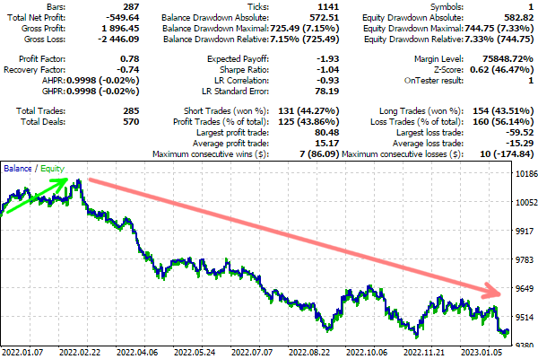
Prediction trading report example

Obviously, for most of 2022, trading was going unsatisfactorily. However, on the left side, immediately after 2021, which was the training dataset, there is a short profitable period. Probably, the patterns found by the network continued to operate for some time. If we wanted to find out whether this is really so, and whether the settings of the network or the training set should be changed in any way in order to improve performance, we would need to conduct comprehensive research for each specific trading system. This is a lot of painstaking work, not related to the internal implementation of neural network algorithms. Here we will only do a minimal analysis.

The log shows the name of the file with the trained network. Specify it in the tester in the NetBinFileName parameter, and expand the testing time, starting from 2021. In this mode, all input parameters, except for the first two (Symbols and Depth), have no meaning.

Test trading on an extended interval shows the following balance dynamics (the training dataset is highlighted in yellow).

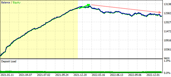
Balance curve when trading on an extended interval, including training set

As expected, the network learned the specifics of a particular interval, but soon after its completion it ceases to be profitable.

Let us repeat the network training twice: with dropout of 25% and 50% (the DropOutPercentage parameter should be set to 25 and then to 50 in sequence). To initiate the training of new networks, clear the NetBinFileName parameter and return the test start date to 2022.01.01.

With the dropout of 25%, we get a noticeably larger error than in the first case. This is an expected result, since we are trying to extend its applicability to out-of-sample data by coarsening the model.

  Epoch 0 of 1000, loss 2.04525 ma(2.04525)
  Epoch 125 of 1000, loss 0.46777 ma(0.48644)
  Epoch 251 of 1000, loss 0.36113 ma(0.36982)
  Epoch 381 of 1000, loss 0.30045 ma(0.30557)
  Epoch 503 of 1000, loss 0.27245 ma(0.27566)
  Epoch 624 of 1000, loss 0.24399 ma(0.24698)
  Epoch 744 of 1000, loss 0.22291 ma(0.22590)
  Epoch 840 of 1000, loss 0.19507 ma(0.20062)
  Epoch 930 of 1000, loss 0.18931 ma(0.19018)
  Done by epoch limit 1000 with accuracy 0.182581
  Training result: 0.18258059873803228

At the dropout of 50%, the error increases even more.

  Epoch 0 of 1000, loss 2.04525 ma(2.04525)
  Epoch 118 of 1000, loss 0.54929 ma(0.55782)
  Epoch 242 of 1000, loss 0.43541 ma(0.45008)
  Epoch 367 of 1000, loss 0.38081 ma(0.38477)
  Epoch 491 of 1000, loss 0.34920 ma(0.35316)
  Epoch 611 of 1000, loss 0.30940 ma(0.31467)
  Epoch 729 of 1000, loss 0.29559 ma(0.29751)
  Epoch 842 of 1000, loss 0.27465 ma(0.27760)
  Epoch 956 of 1000, loss 0.25901 ma(0.26199)
  Done by epoch limit 1000 with accuracy 0.251914
  Training result: 0.25191436104184456

The following figure shows training graphs in three variants.

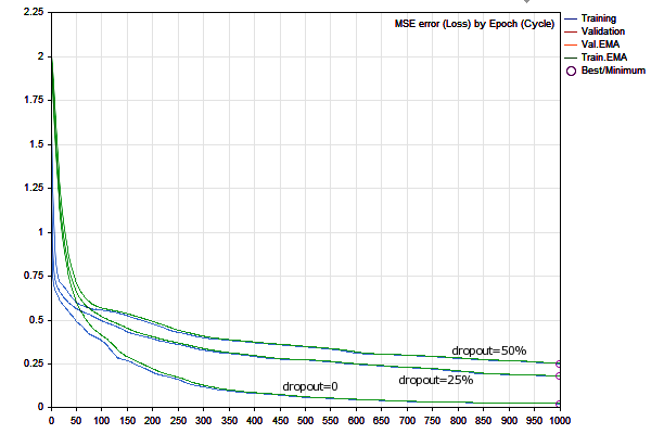
Learning dynamics with different dropout values

Here are the balance curves (the training dataset is highlighted in yellow).

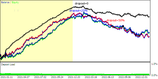
Trading balance curves according to predictions made by networks with different dropouts

Due to the random disconnection of the weights during the dropout, the balance line on the training period becomes not as smooth as with the full network, and the total profit naturally decreases.

In this experiment, all options pretty quickly (within a month or two) lose touch with the market, but the essence of the experiment was to test the created neural network tools rather than to develop a complete system.

In general, the average dropout value of 25% seems to be more optimal, because a smaller degree of regularization leads us back to overfitting, and a larger degree destroys the network's computational capabilities. However, the main conclusion that we can preliminarily draw is that the neural network approach is not a panacea that can "save" any trading system. The failures can be caused by incorrect assumptions about the presence of specific dependencies or by wrong parameters of different algorithm modules or incorrectly prepared data.

Before discarding deciding not to use this (or any other) trading system, you should try various ways to find the best network settings, as it is normally done for EAs without AI. We need to collect more statistics in order to make well-conditioned conclusions.

In particular, we can search for other clusters of symbols or timeframes, run optimization on currently available public variables, or expand their list (for example, by adding activation functions, vector generation methods, filtering by days of the week, etc.).

The use of NN in no way relieves the trader from the need to generate hypotheses, test ideas and significant factors. The only difference is that the optimization of the trading system settings is complemented by NN's metaparameters.

As an experiment, let us run optimizations on vector size, number of vectors, hidden layer size factor and dropout. In addition, we will include the Randomizer parameter in the optimization. This will enable the generation of several instances of networks for each combination of other settings.

• Vector size (Depth) — from 1 to 5
• Training set (Reserve) — from 50 to 400 in increments of 50
• Hidden Layer Factor — from 1 to 5
• DropOut — 0, 25%, 50%
• Randomizer — from 0 to 9

The .set file with the settings is attached below. Date interval is from 2022.01.01 to 2023.02.15.

For the optimization criterion, we will use, for example, Profit Factor. Although, given the small number of combinations (6000) and their complete iterations (unlike genetic optimization), this is not important.

To analyze optimization results, we can export data to an XML file or directly use the .opt file, as described in the OLAP program from the article Quantitative and visual analysis of tester reports or using any other scripts (opt is an open format).

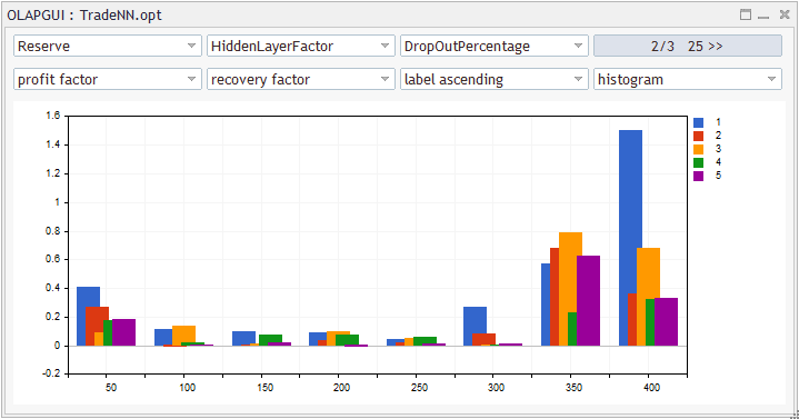
Statistical analysis of the optimization report

For this screenshot, the variables were aggregated in the requested breakdowns (Reserve by X (horizontal axis) relative to HiddenLayerFactor by Y (marked in color) with DropOutPercentage 25% by Z) using a specific profit factor calculation (by cells in the X/Y/Z axes) from the recovery factor (from each pass of the tester during the optimization). Such an artificial quality measure is not ideal, but it is available out of the box.

Similar or more familiar statistics can be calculated in Excel.

Statistically better performance was achieved with a hidden layers factor of 1 (instead of 2, as it was by default), and a vector size of 4 (instead of 5). The recommended dropout value is 25% or 50%, but not 0%.

Also, as expected, a deeper history is preferable (350 or 400 counts and probably a further increase is justified).

Let us summarize the found working settings:

• Vector size = 4
• Training set = 400
• Hidden Layer Factor = 1

Since the Randomizer parameter was used in the optimization, we have 30 network instances trained in this configuration: 10 networks for each dropout level (0%, 25%, 50%). We need 25% and 50%. By uploading the optimization report in XML, we can filter the necessary records and get a table (sorted by profitability with a filter greater than 1):

Pass    Result  Profit  Expected Profit  Recovery Sharpe Custom  Equity Trades Depth  Reserve Hidden  DropOut Randomizer
			Payoff	 Factor	 Factor	 Ratio	 	 DD %			      LayerF	Perc
3838    1.35    336.02  2.41741  1.34991 1.98582 1.20187 1       1.61    139     4       400     1       25      6
838     1.23    234.40  1.68633  1.23117 0.81474 0.86474 1       2.77    139     4       400     1       25      1
3438    1.20    209.34  1.50604  1.20481 0.81329 0.78140 1       2.47    139     4       400     1       50      5
5838    1.17    173.88  1.25094  1.16758 0.61594 0.62326 1       2.76    139     4       400     1       50      9
5038    1.16    167.98  1.20849  1.16070 0.51542 0.60483 1       3.18    139     4       400     1       25      8
3238    1.13    141.35  1.01691  1.13314 0.46758 0.48160 1       2.95    139     4       400     1       25      5
2038    1.11    118.49  0.85245  1.11088 0.38826 0.41380 1       2.96    139     4       400     1       25      3
4038    1.10    107.46  0.77309  1.09951 0.49377 0.38716 1       2.12    139     4       400     1       50      6
1438    1.10    104.52  0.75194  1.09700 0.51681 0.37404 1       1.99    139     4       400     1       25      2
238     1.07    73.33   0.52755  1.06721 0.19040 0.26499 1       3.69    139     4       400     1       25      0
2838    1.03    34.62   0.24907  1.03111 0.10290 0.13053 1       3.29    139     4       400     1       50      4
2238    1.02    21.62   0.15554  1.01927 0.05130 0.07578 1       4.12    139     4       400     1       50      3

Let us take the best one, the first line.

During optimization, all trained networks are saved in the MQL5/Files/<expert name>/<optimization date> folder. Actually, this can be omitted, given that a similar network can be re-trained by the Randomizer value, but only if the input data fully matches. If the history of quotes changes (for example, you use another broker), it will not be possible to reproduce the network with exactly these characteristics.

The files in the specified folder have names consisting of the names and values of the optimized parameters. So, you can simply search the file system:

Depth=4-Reserve=400-HiddenLayerFactor=1-DropOutPercentage=25-Randomizer=6

Let's say the file is named:

Depth=4-Reserve=400-HiddenLayerFactor=1-DropOutPercentage=25-Randomizer=6-3838(0.428079).bpn

where the number in parentheses is the network error, the number in front of the brackets is the pass number.

Let us look inside the file: despite the fact that the file is binary, our training metadata is saved as text at its end. So, we see that the training interval was 2021.01.12 00:00-2022.07.28 00:00 (400 bars D1 ).

We copy the file under a shorter name, for example, test3838.bpn, to the common terminal folder.

Specify the name test3838.bpn in the NetBinFileName parameter and set the 'Vector size' (Depth) to 4 (all other parameters do not matter if we only work in the forecasting mode).

Let us check the EA trading on an even longer period: since 2022-2023 were used as a validation forward test, we will capture 2020 as an unknown period.

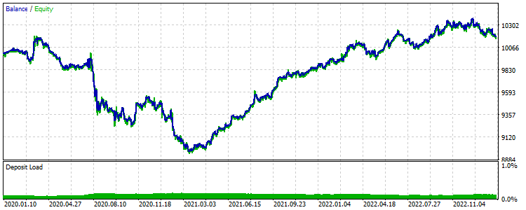
An example of a failed prediction trading test outside the training set

The miracle did not happen: the system is also unprofitable on new data. This picture would be similar for other settings as well.

So, we have two news: good and bad.

The bad news is that the proposed idea does not work — it either doesn’t work at all or it is due to the limitations of the examined factor space in our demo (since we didn’t run super-mega-optimization for billions of combinations and hundreds of symbols).

The good news is that the proposed neural network toolkit can be used to evaluate ideas and produces the expected (from a technical point of view) results.

Conclusion

This article presents backpropagation neural networks classes using MQL5 matrices. The implementation does not depend on external programs, such as Python, and does not require special firmware (graphic accelerators with OpenCL support). In addition to regular neural network training and operation modes, the classes provide capabilities for visualization of the process, as well as for saving and restoring networks in files.

With these classes, the use of neural networks can be quite easily integrated into any program. However, please note that the network is just a tool applied to some material (in our case: financial data). If the material does not contain enough information, is very noisy or irrelevant, no neural network will be able to find the grail in it.

The backpropagation algorithm is one of the most common basic learning methods, which can be used as the basis to construct more complex neural network technologies, such as recurrent networks, convolutional networks and reinforcement learning.