Practical application of neural networks in trading (Part 2). Computer vision
Introduction
An essential problem in preparing data to training neural networks designed for trading, is related the preparation of the necessary input data. For example, consider the case when we use a dozen indicators. These indicators may represent a set of several informative charts. If we calculate these indicators to a certain depth, then as a result we will get up to a hundred entries, and in some cases even more. Can we make neural network training easier by using computer vision? To solve this problem, let us use convolutional neural networks, which are often utilized to solve classification and recognition problems.
Convolutional neural network architecture
In this article, we will use a convolutional neural network. Its architecture is shown in the figure below. This scheme shows the general principle for constructing a Convolutional Neural Network (CNN).
In this case, we have:
- CNN input, which is an image of size 449x449 pixels.
- The first convolutional layer of 96 feature maps. Each map is an image of size 447x447. Convolution kernel 3x3.
- Subsample layer of 96 feature maps with a size of 223x223, with a kernel 2x2.
- Second convolutional layer of 32 feature maps. Each map is an image of size 221x221. Convolution kernel 3x3.
- Subsample layer of 32 feature maps with a size of 110x110, with a kernel 2x2.
- Third convolutional layer of 16 feature maps. Each map is an image of size 108x108. Convolution kernel 3x3.
- Subsample layer of 16 feature maps with a size of 54x54, with a kernel 2x2. Not shown in the figure.
- Fully connected layer of 64 neurons.
- Output layer of one neuron. These two layers represent the classification unit.

If you are new to convolutional neural networks, do not worry about the seeming cumbersomeness and complexity of construction. A neural network of a given architecture is built automatically. You only need to set the main parameters.
Preparing an array of images for neural network training and testing
Before preparing an array of images, define the purpose of your neural network. Ideally, it would be great to train the network at pivots. According to this purpose, we would need to make screenshots with the last extreme bar. However, this experiment showed no practical value. That is why we will use another set of images. Further, you can experiment with different arrays, including the above mentioned one. This may also provide additional proofs of the efficiency of neural networks in solving image-based classification tasks. The neural network responses obtained on a continuous time series require additional optimization.
Let us not complicate the experiment and focus on two categories of images:
- Buy - when the price moves up or when the price has reached the daily low
- Sell - when the price moves down or when the price has reached the daily high
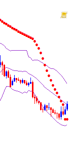
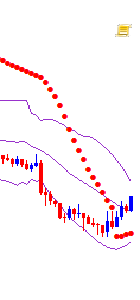
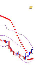
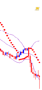
For neural network training purposes, the movement in any direction will be determined as the price reaching new extreme values in trend direction. At these moments chart screenshots will be made. Trend reversal moment is also important for network training. A chart screenshot will also be made when the price reaches the daily high or low.
Before starting operation, we need to prepare the chart appearance. Use the CNN.tpl template. Save it to \AppData\Roaming\MetaQuotes\Terminal\D0E8209F77C8CF37AD8BF550E51FF075\MQL5\Profiles\Templates.
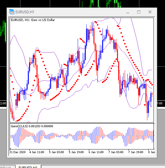
Define the text as "White" in chart properties.
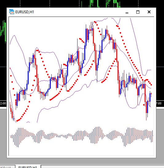
You can also attach any other indicators. I took these indicators arbitrary. It is also recommended to find an optimal chart size according to your hardware capabilities.
Use the following script for creating an array of images.
//+------------------------------------------------------------------+
//|                                                        CNNet.mq5 |
//|                                   Copyright 2021, Andrey Dibrov. |
//|                           https://www.mql5.com/en/users/tomcat66 |
//+------------------------------------------------------------------+
#property copyright "Copyright 2021, Andrey Dibrov."
#property link      "https://www.mql5.com/en/users/tomcat66"
#property version   "1.00"
#property strict
#property script_show_inputs

input string Date="2017.01.02 00:00";
input string DateOut="2018.12.13 23:00";
input string DateTest="2019.01.02 00:00";
input string Dataset="Train";

string Date1;
int count,countB,countS;
int day;
double DibMin;
double DibMax;
int HandleDate;
long WIDTH;
long HEIGHT;
//+------------------------------------------------------------------+
//| Script program start function                                    |
//+------------------------------------------------------------------+
void OnStart()
  {
//---
   MqlDateTime stm;
   ChartSetInteger(0,CHART_SHIFT,false);
   ChartSetInteger(0,CHART_AUTOSCROLL,false);
   ChartSetInteger(0,CHART_SHOW_OBJECT_DESCR,false);
   WIDTH=ChartGetInteger(0,CHART_WIDTH_IN_PIXELS);
   ChartSetInteger(0,CHART_SHOW_PRICE_SCALE,false);

   if(Dataset=="Test")
     {
      HandleDate=FileOpen(Symbol()+"Date.csv",FILE_CSV|FILE_READ|FILE_WRITE|FILE_ANSI,";");
      ChartNavigate(0,CHART_END,-(iBarShift(NULL,PERIOD_H1,StringToTime(DateTest))));
      Sleep(1000);

      for(int i=iBarShift(NULL,PERIOD_H1,StringToTime(DateTest)); i>0; i--)
        {
         Date1=TimeToString(iTime(NULL,PERIOD_H1,i));
         if(DateTest<=Date1)
           {
            if(ChartNavigate(0,CHART_END,-i))
              {
               Sleep(20);
               if(ChartScreenShot(0, (string)count + ".png", (int)WIDTH, (int)WIDTH, ALIGN_LEFT))
                 {
                  FileWrite(HandleDate,TimeToString(iTime(NULL,PERIOD_H1,i)));
                  count++;
                  Sleep(20);
                 }
              }
           }
        }
     }
   if(Dataset=="Train")
     {
      ChartNavigate(0,CHART_END,-iBarShift(NULL,PERIOD_H1,StringToTime(Date)));
      Sleep(1000);
      for(int i=iBarShift(NULL,PERIOD_H1,StringToTime(Date)); i>=iBarShift(NULL,PERIOD_H1,StringToTime(DateOut)); i--)
        {
         TimeToStruct(iTime(NULL,PERIOD_H1,i),stm);
         Date1=TimeToString(iTime(NULL,PERIOD_H1,i));
         if(DateOut>=Date1 && Date<=Date1)
           {
            if(ChartNavigate(0,CHART_END,-i))
              {
               Sleep(20);
               if(day != stm.day)
                 {
                  FileCopy("Sell" + (string)countS + ".png", 0, "Buy" + (string)(countB+1) + ".png", FILE_REWRITE);
                  FileDelete("Sell" + (string)countS + ".png", 0);
                  FileCopy("Buy" + (string)countB + ".png", 0, "Sell" + (string)(countS+1) + ".png", FILE_REWRITE);
                  FileDelete("Buy" + (string)countB + ".png", 0);
                  countB ++;
                  countS ++;
                 }
               day = stm.day;
               if(stm.hour == 0)
                 {
                  DibMin = iOpen(NULL, PERIOD_H1, i);
                  DibMax = iOpen(NULL, PERIOD_H1, i);
                 }
               if(iLow(NULL, PERIOD_H1, i+1) < DibMin)
                 {
                  DibMin = iLow(NULL, PERIOD_H1, i+1);
                  countS ++;
                  ChartScreenShot(0, "Sell" + (string)countS + ".png", (int)WIDTH, (int)WIDTH, ALIGN_LEFT);
                 }
               if(iHigh(NULL, PERIOD_H1, i+1) > DibMax)
                 {
                  DibMax = iHigh(NULL, PERIOD_H1, i+1);
                  countB ++;
                  ChartScreenShot(0, "Buy"  +(string)countB + ".png", (int)WIDTH, (int)WIDTH, ALIGN_LEFT);
                 }
               Sleep(20);
              }
           }
         else
            break;
        }
     }
  }
The script works in two modes: "Train" — creates an array of images for training, and "Test" — creates an array of images for obtaining neural network responses, based on which an indicator will be generated. Further this indicator will be used for optimizing the trading strategy.
Let us run the script in the "Train" mode.
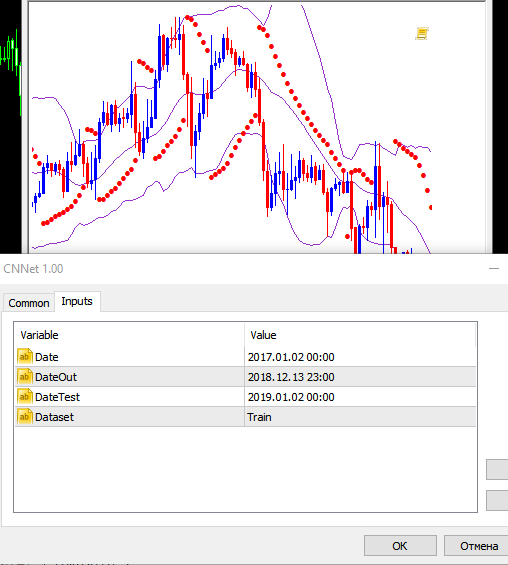
Variable "Date" — initial data for the sample in which images for training will be selected. "DateOut' — the end date of the sample period in which images for training will be selected. "DateTest" — the starting date for selecting images to obtain hourly responses from the neural network. The end date will be the script launch hour.
A set of Buy... and Sell... images will be saved in the ...\MQL5\Files folder of the data directory. The total number of images is 6125.
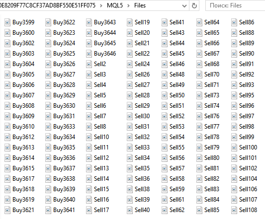
Next, prepare directories for the training, validation and testing set. For convenience, create the "CNN" folder on the Desktop, and create three folders in it - "Train", "Val", "Test".

In "Train" and "Val" directories, create subdirectories "Buy" and "Sell". Create a subdirectory "Resp" under "Test".

From the folder ...\MQL5\Files, cut all files "Buy..." and past them to ...\Train\Buy. We have 3139 images. Repeat the same for "Sell..." and add them to ...\Train\Sell. Here we have 2986 images. From folders "Buy" and "Sell", cut 30% of last (having the highest numbers) images and past them to the appropriate subfolders under "Val".
What we have now
- ...\Train\Buy - 2198 images
- ...\Val\Buy - 941 images
- ...\Train\Sell - 2091 images
- ...\Val\Sell - 895 images
We have prepared a set of images for training the network. I got images of size 449x449 pixels.
Prepare a set of images for testing. Run the script in the "Test" mode.
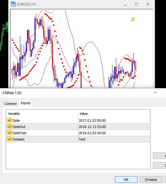
A set of sequential hourly screenshots will be saved to ...\MQL5\Files. They are 12558 now. Do not separate or group them, as the neural network should perform this grouping by itself. To be more precise, the network should show the probability of that an image corresponds to the conditions under which the network was trained. Upward move and turn down. Downward move and turn up.
Cut these files and past to ...CNN\Test\Resp.
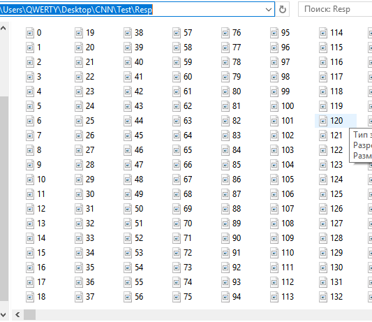
We have prepared a set of images for testing the responses and optimizing the strategy. The files with date and time EURUSDDate, remaining under ...\MQL5\Files, should be moved to the CNN folder.
I would like to note one specific feature of MetaTrader 5. It would be more convenient and reliable to prepare a set of images using an Expert Advisor in the strategy tester. However, MetaTrader 5 does not provide the ability to create screenshots in the strategy tester. Anyway, this specific feature will not affect trading robot creation.
Training the neural network
We will work with convolutional networks using the Anaconda environment. It should be configured to work with CPU and GPU (if you have an NVIDIA graphics card). This graphics card is needed to speed up the learning process. Although, it imposes some restrictions in creating a neural network architecture - dependence on the amount of RAM of the graphics card. But the learning speed is increased significantly. For example, in my case, one training epoch on a CPU lasts 20 minutes, and it takes 1-2 minutes on a GPU. If the network is trained on 40 epochs, then I would have 13 and 1.5 hours. The usage of GPU can significantly speed up the neural network search process at the research stage.
- Download and install the latest Anaconda Navigator version. Use default settings at all steps.
- Launch "Anaconda Prompt" using menu "Start\Anaconda3".
- Run the command "pip install tensorflow". Install the program library for machine learning developed by Google.
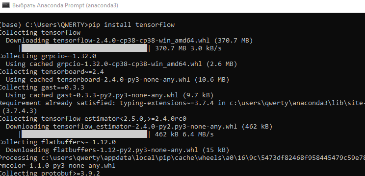
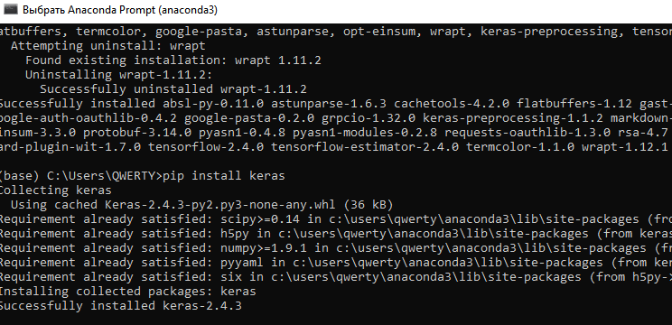
- Run command "pip install keras". Install the Keras neural network library.
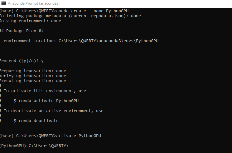
- Create a new 'conda' environment under GPU. Type command conda create --name PythonGPU. Activate the environment - activate PythonGPU.
-
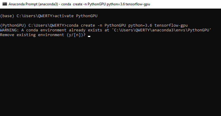
To install tensorflow gpu type the command conda create -n PythonGPU python=3.6 tensorflow-gpu. Please note that tensorflow gpu should be installed for python 3.6.
-
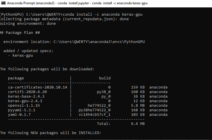
To install keras gpu, type the command conda install -c anaconda keras-gpu.
-
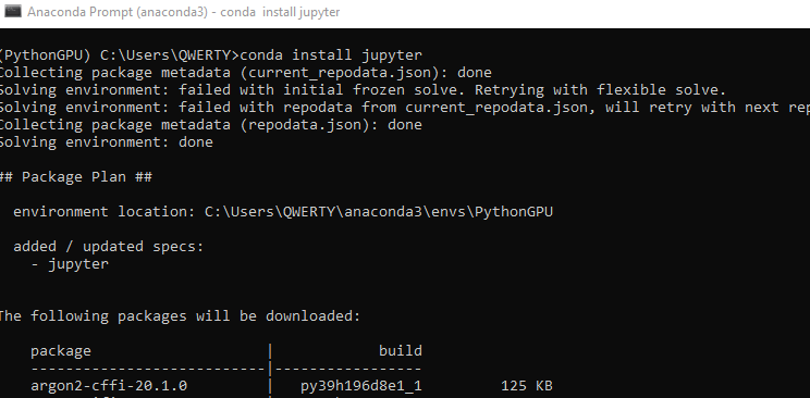
Install the Jupyter interface for programming in the Python GPU environment. CPU Jupyter was already installed during Anaconda installation. Type command - conda install jupyter.
-
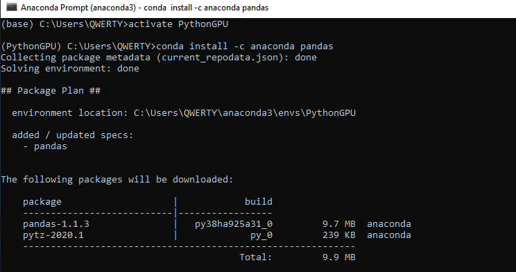
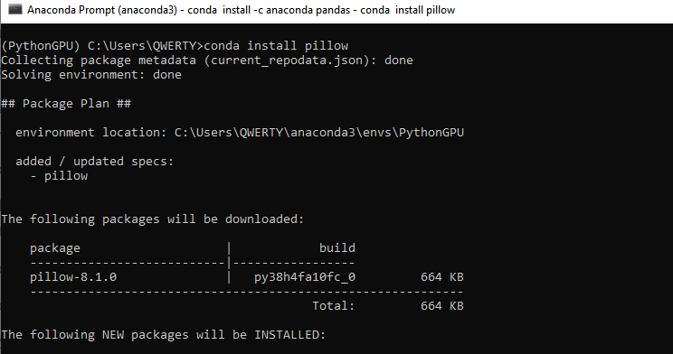
Install two more libraries, Pandas and Pillow - conda install -c anaconda pandas. Then - conda install pillow. These libraries should also be installed for CPU if you are not going to use a graphics card.
-
- We can now start training our convolutional neural network. Add two files to the previously created CNN folder: Train.ipynb and Test.ipynb. These are files in the Jupyter Notebook format, with which we will work. Run Jupyter Notebook (PythonGPU) and open file Train.
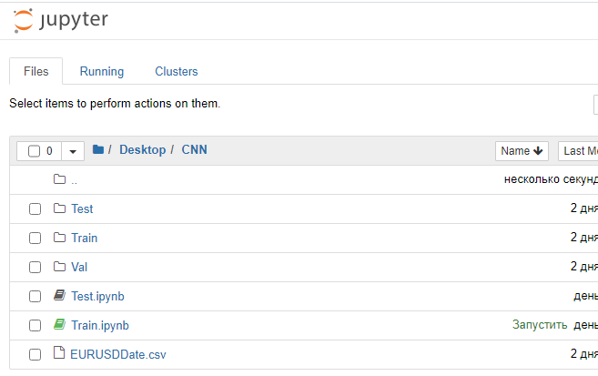
Let us consider every block of the program code.
First load the necessary modules of neural network libraries.
from tensorflow.python.keras.preprocessing.image import ImageDataGenerator
from tensorflow.python.keras.models import Sequential
from tensorflow.python.keras.layers import Conv2D, MaxPooling2D
from tensorflow.python.keras.layers import Activation, Dropout, Flatten, Dense
from tensorflow.keras.callbacks import ModelCheckpoint
from tensorflow.keras.models import load_model
Then set the required hyperparameters.
# Directory with data for training
train_dir = 'train'
# Directory with data for validation
val_dir = 'val'
# Image dimensions
img_width, img_height = 449, 449
# Image-based tensor dimension for input to the neural network
# backend Tensorflow, channels_last
input_shape = (img_width, img_height, 3)
# Number of epochs
epochs = 20
# Mini-sample size
batch_size = 7
# Number of images for training
nb_train_samples = 4289
# Number of images for validation
nb_validation_samples = 1836
# Number of images for testing
#nb_test_samples = 3736
Let us create the network architecture.
- Set a sequential convolutional neural network architecture
- The input image is of size 449x449 pixels, three-channel (red, green and blue). Here we use a color image. You can also try a monochrome image
- Create the first convolution layer for working with two-dimensional data: 96 feature maps each having it sown 3x3 convolution kernel. Each neuron of the convolutional layer is connected to a 3x3 square section of the image
- Activation layer using the "relu" function, which is less computationally intensive
- To reduce the dimension, add a subsampling layer with a 2x2 kernel with the selection of the maximum value from this square
- Next, add two more convolution layers with 32 and 16 cores, two activation layers and two subsamples
- Converting two-dimensional data to one-dimensional format
- Pass the converted data to the fully connected layer having 64 neurons
- Using the Dropout(0.5) regularization layer function try to avoid overfitting
- Add a fully connected output layer with one neuron. Two image classes are used, so network response will be received in a binary response. It is also possible to try several classes. For example, two for trend and one for flat. In this case, the output layer would have three neurons. Also, we would need to divide images into three classes.
- The "sigmoid" activation function. It is good for classification and it has shown the best performance during my experiments
This example of architecture can be easily modernized - we can increase the number of layers and their sizes, change their position depending on the sequence, change the dimension of the convolution kernel, modify activation functions and work with fully connected layers. However, a dilemma arises here: when using a GPU, it is necessary to increase the RAM of a video card in case we want to increase the architecture of a neural network. Optionally, the image size should be reduced. Otherwise, we can spend a lot of time using CPU.
model = Sequential()
model.add(Conv2D(96, (3, 3), input_shape=input_shape))
model.add(Activation('relu'))
model.add(MaxPooling2D(pool_size=(2, 2)))

model.add(Conv2D(32, (3, 3)))
model.add(Activation('relu'))
model.add(MaxPooling2D(pool_size=(2, 2)))

model.add(Conv2D(16, (3, 3)))
model.add(Activation('relu'))
model.add(MaxPooling2D(pool_size=(2, 2)))

model.add(Flatten())
model.add(Dense(64))
model.add(Activation('relu'))
model.add(Dropout(0.5))
model.add(Dense(1))
model.add(Activation('sigmoid'))
Compile the neural network. Use the error function: binary-crossentropy. In this case, we will use a response consisting of two classes which should take the values 0 or 1, ideally. However, actual values will be distributed from 0 to 1. Select the Gradient Descent optimizer. It seems to be the most suitable for neural network training. Choose the accuracy metric, i.e. the percentage of correct answers.
model.compile(loss='binary_crossentropy',
              optimizer='sgd',
              metrics=['accuracy'])
Normalize the data on the intensity of image pixels.
datagen = ImageDataGenerator(rescale=1. / 255)
Use Keras generators to read data from the disk and to create the training and validation image arrays for the neural network. Again, class_mode is 'binary'. Set Shuffle to 'False'. So, image shuffling is disabled.
train_generator = datagen.flow_from_directory(
    train_dir,
    target_size=(img_width, img_height),
    batch_size=batch_size,
    class_mode='binary',
    shuffle=False)
val_generator = datagen.flow_from_directory(
    val_dir,
    target_size=(img_width, img_height),
    batch_size=batch_size,
    class_mode='binary',
    shuffle=False)
The callbacks function saves the trained neural network after each epoch. This allows selecting the most suitable network in terms of error values and hit percentage.
callbacks = [ModelCheckpoint('cnn_Open{epoch:1d}.hdf5')] Now, proceed to network training.
model.fit(
    train_generator,
    steps_per_epoch=nb_train_samples // batch_size,
    epochs=epochs,
    validation_data=val_generator,
    validation_steps=nb_validation_samples // batch_size,
    callbacks=callbacks)
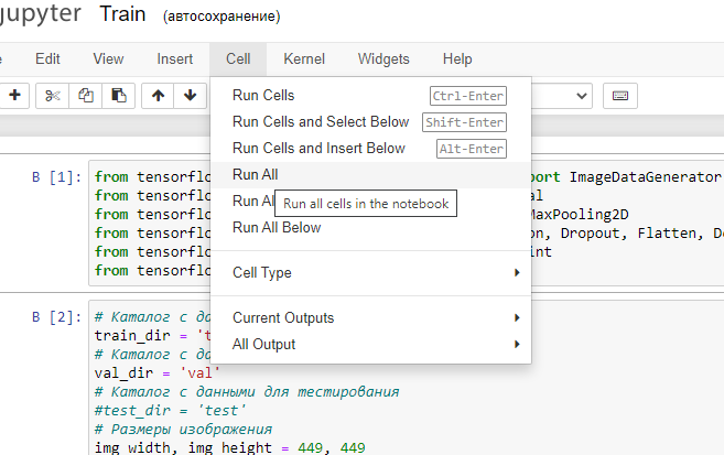
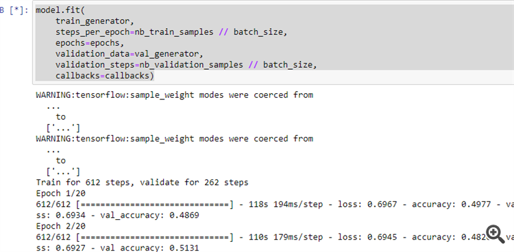
12. Run the program as shown in the figure.
If the previous steps have been performed correctly, the neural network will start learning.
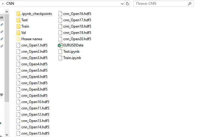
After the end of the training process, 20 trained neural networks will appear under the CNN folder.
Let us view training results and select a neural network for further use.
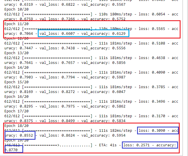
At first glance, at epoch 18 the neural network learned with an error rate of 30% and with 85% correct results. However, when running the neural network on the validation set, we see that the error grows, and the percentage of correct answers falls. SO, we should select a network trained at epoch 11. It has the most suitable results at the validation set: val_loss = 0.6607 and val_accuracy = 0.6129. Ideally, the error value should tend to 0 (or at least no more than 35-40%), while the accuracy should be close to 1 (at least no less than 55-60%). In this case optimization could be omitted or could be performed by minimum parameters to improve trading quality. Even with these training results it is possible to create a profitable trading system.
Interpreting the neural network response
Let us now check if all the above work has any practical meaning.
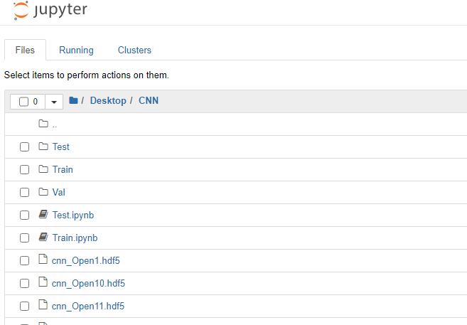
Run Jupyter Notebook without GPU support and open Test.jpynb from the CNN directory.
Let us consider the code blocks.
First load the necessary modules of neural network libraries.
from tensorflow.python.keras.preprocessing.image import ImageDataGenerator
from tensorflow.python.keras.models import Sequential
from tensorflow.python.keras.layers import Conv2D, MaxPooling2D
from tensorflow.python.keras.layers import Activation, Dropout, Flatten, Dense
from tensorflow.keras.callbacks import ModelCheckpoint
from tensorflow.keras.models import load_model
import pandas as pd
Set required parameters.
predict_dir = 'Test'
img_width, img_height = 449, 449
nb_predict_samples = 12558
Read data and time of tested images from the file.
Date=pd.read_csv('EURUSDDate.csv', delimiter=';',header=None) Load the neural network saved after the 11th epoch.
model=load_model('cnn_Open11.hdf5') Normalize the images.
datagen = ImageDataGenerator(rescale=1. / 255)
Read data from the disk using the generator.
predict_generator = datagen.flow_from_directory(
    predict_dir,
    target_size=(img_width, img_height),
    shuffle=False)
Get responses from the neural network.
indicator=model.predict(predict_generator, nb_predict_samples )
Show the result. Feedback obtaining process takes much time, so below is a notification of process completion.
print(indicator)
Save the obtained result to a file.
Date=pd.DataFrame(Date)
Date['0'] =indicator
Date.to_csv('Indicator.csv',index=False, header=False,sep=';')
Run the program. Once it is complete, the Indicator.csv file will be created under the CNN directory.
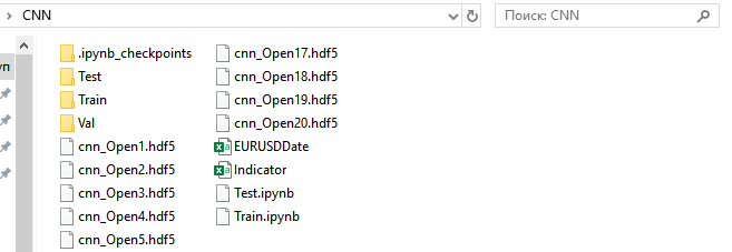
Move it to C:\Users\...\AppData\Roaming\MetaQuotes\Terminal\Common\Files.
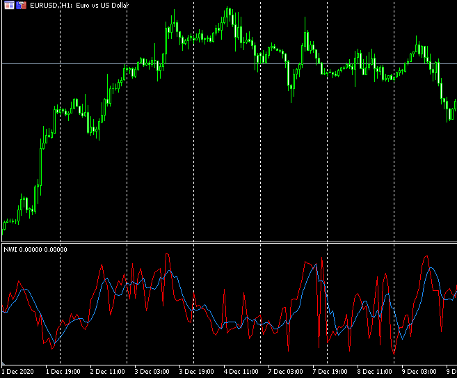
Run indicator NWI on the EURUSD H1 chart.
//+------------------------------------------------------------------+
//|                                                          NWI.mq5 |
//|                                 Copyright © 2019, Andrey Dibrov. |
//+------------------------------------------------------------------+
#property copyright "Copyright © 2019, Andrey Dibrov."
#property link      "https://www.mql5.com/en/users/tomcat66"
#property version   "1.00"
#property indicator_separate_window
#property indicator_buffers 2
#property indicator_plots   2
#property indicator_type1   DRAW_LINE
#property indicator_type2   DRAW_LINE
#property indicator_color1  Red
#property indicator_color2  DodgerBlue


int Handle;
int i;
int h;
input int Period=5;
double    ExtBuffer[];
double    SignBuffer[];
datetime Date1;
datetime Date0;
string File_Name="Indicator.csv";

//+------------------------------------------------------------------+
//| Custom indicator initialization function                         |
//+------------------------------------------------------------------+
void OnInit()
  {
   SetIndexBuffer(0,ExtBuffer,INDICATOR_DATA);
   SetIndexBuffer(1,SignBuffer,INDICATOR_DATA);
   IndicatorSetInteger(INDICATOR_DIGITS,5);
   Handle=FileOpen(File_Name,FILE_CSV|FILE_SHARE_READ|FILE_ANSI|FILE_COMMON,";");
   //FileClose(Handle);
  }
//+------------------------------------------------------------------+
//| Relative Strength Index                                          |
//+------------------------------------------------------------------+
int OnCalculate(const int rates_total,
                const int prev_calculated,
                const int begin,
                const double &price[])
  {
   MqlDateTime stm;
   Date0=StringToTime(FileReadString(Handle));
   i=iBarShift(NULL,PERIOD_H1,Date0,false);
   Handle=FileOpen(File_Name,FILE_CSV|FILE_SHARE_READ|FILE_ANSI|FILE_COMMON,";");
   ArraySetAsSeries(ExtBuffer,true);
   ArraySetAsSeries(SignBuffer,true);
   while(!FileIsEnding(Handle) && !IsStopped())
     {
      Date1=StringToTime(FileReadString(Handle));
      ExtBuffer[i]=StringToDouble(FileReadString(Handle));
      h=Period-1;
      if(i>=0)
        {
         while(h>=0)
           {
            SignBuffer[i]=SignBuffer[i]+ExtBuffer[i+h];
            h--;
           }
        }
      SignBuffer[i]=SignBuffer[i]/Period;
      TimeToStruct(Date1,stm);
      i--;
     }
   FileClose(Handle);
   return(rates_total);
  }
//+------------------------------------------------------------------+
For simplicity, we will interpret the network responses using the intersection of the main indicator line with a simple average line. Use the TestCNN Expert Advisor.
//+------------------------------------------------------------------+
//|                                                      TestCNN.mq5 |
//|                                 Copyright © 2019, Andrey Dibrov. |
//+------------------------------------------------------------------+
#property copyright " Copyright © 2019, Andrey Dibrov."
#property link      "https://www.mql5.com/en/users/tomcat66"
#property version   "1.00"
#property strict

#include<Trade\Trade.mqh>

CTrade  trade;

input int Period=5;
input int H1;
input int H2;
input int H3;
input int H4;
input int LossBuy;
input int ProfitBuy;
input int LossSell;
input int ProfitSell;

ulong TicketBuy1;
ulong TicketSell0;

datetime Count;

double Per;
double Buf_0[];
double Buf_1[];
bool send1;
bool send0;

int h=4;
int k;
int K;
int bars;
int Handle;
//+------------------------------------------------------------------+
//| Expert initialization function                                   |
//+------------------------------------------------------------------+
int OnInit()
  {
//---

   Handle=FileOpen("Indicator.csv",FILE_CSV|FILE_SHARE_READ|FILE_ANSI|FILE_COMMON,";");

   while(!FileIsEnding(Handle)&& !IsStopped())
     {
      StringToTime(FileReadString(Handle));
      bars++;
     }
   FileClose(Handle);
   ArrayResize(Buf_0,bars);
   ArrayResize(Buf_1,bars);
   Handle=FileOpen("Indicator.csv",FILE_CSV|FILE_SHARE_READ|FILE_ANSI|FILE_COMMON,";");

   while(!FileIsEnding(Handle)&& !IsStopped())
     {
      Count=StringToTime(FileReadString(Handle));
      Buf_0[k]=StringToDouble(FileReadString(Handle));
      h=Period-1;
      if(k>=h)
        {
         while(h>=0)
           {
            Buf_1[k]=Buf_1[k]+Buf_0[k-h];
            h--;
           }
         Buf_1[k]=Buf_1[k]/Period;
        }
      k++;
     }
   FileClose(Handle);

   int deviation=10;
   trade.SetDeviationInPoints(deviation);
   trade.SetTypeFilling(ORDER_FILLING_RETURN);
   trade.SetAsyncMode(true);

//---
   return(INIT_SUCCEEDED);
  }

//+------------------------------------------------------------------+
//| Expert deinitialization function                                 |
//+------------------------------------------------------------------+
void OnDeinit(const int reason)
  {
//---

  }
//+------------------------------------------------------------------+
//| Expert tick function                                             |
//+------------------------------------------------------------------+
void OnTick()
  {
//---
   MqlDateTime stm;
   TimeToStruct(TimeCurrent(),stm);

   int    digits=(int)SymbolInfoInteger(_Symbol,SYMBOL_DIGITS);
   double point=SymbolInfoDouble(_Symbol,SYMBOL_POINT);
   double PriceAsk=SymbolInfoDouble(_Symbol,SYMBOL_ASK);
   double PriceBid=SymbolInfoDouble(_Symbol,SYMBOL_BID);

   double SL1=NormalizeDouble(PriceBid-LossBuy*point,digits);
   double TP1=NormalizeDouble(PriceAsk+ProfitBuy*point,digits);
   double SL0=NormalizeDouble(PriceAsk+LossSell*point,digits);
   double TP0=NormalizeDouble(PriceBid-ProfitSell*point,digits);

   if(LossBuy==0)
      SL1=0;

   if(ProfitBuy==0)
      TP1=0;

   if(LossSell==0)
      SL0=0;

   if(ProfitSell==0)
      TP0=0;

//---------Buy1
   if(send1==false && K>0 && Buf_0[K-1]>Buf_1[K-1] && Buf_0[K]<Buf_1[K] && iLow(NULL,PERIOD_H1,1)<iLow(NULL,PERIOD_H1,2) && stm.hour>H1 && stm.hour<H2 && H1<H2)
     {
      send1=trade.PositionOpen(_Symbol,ORDER_TYPE_BUY,1,PriceAsk,SL1,TP1);
      TicketBuy1 = trade.ResultDeal();
     }

   if(send1==true && K>0 && Buf_0[K-1]<Buf_1[K-1] && Buf_0[K]>Buf_1[K] && iHigh(NULL,PERIOD_H1,1)>iHigh(NULL,PERIOD_H1,2))
     {
      trade.PositionClose(TicketBuy1);
      send1=false;
     }

//---------Sell0

   if(send0==false && K>0 && Buf_0[K-1]<Buf_1[K-1] && Buf_0[K]>Buf_1[K] && iHigh(NULL,PERIOD_H1,1)>iHigh(NULL,PERIOD_H1,2) && stm.hour>H3 && stm.hour<H4 && H3<H4)
     {
      send0=trade.PositionOpen(_Symbol,ORDER_TYPE_SELL,1,PriceBid,SL0,TP0);
      TicketSell0 = trade.ResultDeal();
     }

   if(send0==true && K>0 && Buf_0[K-1]>Buf_1[K-1] && Buf_0[K]<Buf_1[K] && iLow(NULL,PERIOD_H1,1)<iLow(NULL,PERIOD_H1,2))
     {
      trade.PositionClose(TicketSell0);
      send0=false;
     }
   K++;
  }
//+------------------------------------------------------------------+
Let us optimize simultaneously by the signal line period, time and stop orders for deals in both directions.
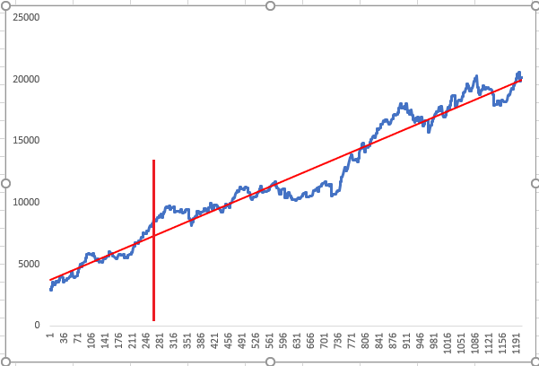
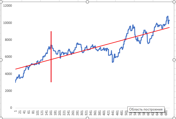
The neural network was trained on a time period preceding the chart line, and optimization was performed up to the vertical red line. Then test was performed for optimized neural network responses. The above charts show two random positive optimization results, which the optimizer has shown as the highest priority result.
Visualizing neural network layers and improving CNN quality
The neural network may seem to be a kind of black box. However, this is not quite so, since we can view which features the neural network is highlighting in feature maps in layers. This provides information for further analysis and network quality improvement. Let us have a look.
Run Visual.ipynb from the CNN folder.
First load the necessary modules of neural network libraries.
from tensorflow.python.keras.preprocessing.image import ImageDataGenerator
from tensorflow.keras.models import Model, load_model
import pandas as pd
from tensorflow.python.keras.preprocessing import image
import matplotlib.pyplot as plt
import numpy as np
Load the saved model.
model=load_model('cnn_Open11.hdf5') Let us take a look at the network architecture.
model.summary()
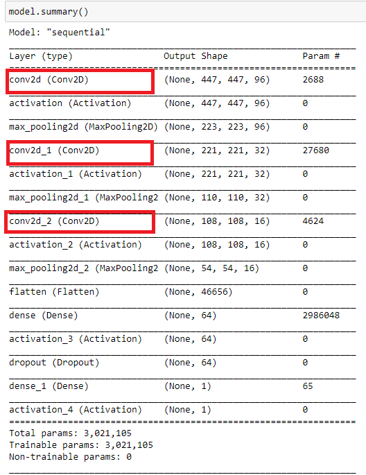
What do these convolutional layers analyze?
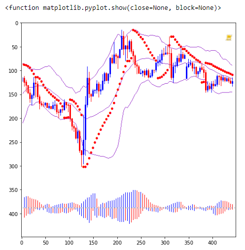
Load some image.
img_path='Train/Buy/Buy81.png'
img=image.load_img(img_path,target_size=(449,449))
plt.figure(figsize=(8, 8))
plt.imshow(img)
plt.show
Convert the image to a numpy array and normalize.
x=image.img_to_array(img)
x=np.expand_dims(x,axis=0)
x/=255
Crop the model on some convolutional layer. Convolutional layer numbers are 0, 3, 6. Start from zero. In fact, we create a new already trained model, from which we will receive an intermediate result before classification.
model=Model(inputs=model.input, outputs=model.layers[0].output)
After that we can view layers 3 and 6.
#model=Model(inputs=model.input, outputs=model.layers[3].output)
#model=Model(inputs=model.input, outputs=model.layers[6].output)
Show information about the cropped model.
model.summary()
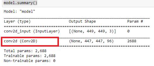
Check the first convolutional layer 0.
Get neural network response.
model=model.predict(x)
Print one of the feature maps, 18.
print(model.shape)
im=model[0,:,:,18]
plt.figure(figsize=(10, 10))
plt.imshow(im)
plt.show()
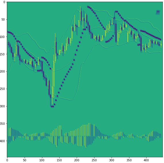
As you can see, the network has highlighted here bullish candlesticks. At this stage, it is hard for the neural network to distinguish between bearish candlesticks and Parabolic points. This is because the same color is used for them. So, all elements of the chart should be presented in different colors.
Check all feature maps
rows=12
filters=model.shape[-1]
size=model.shape[1]
cols=filters//rows
display_grid=np.zeros((cols*size,rows*size))
for col in range(cols):
    for row in range(rows):
        channel_image=model[0,:,:,col*rows+row]
        channel_image-=channel_image.mean()
        channel_image/=channel_image.std()
        channel_image*=64
        channel_image+=128
        channel_image=np.clip(channel_image,0,255).astype('uint8')
        display_grid[col*size:(col+1)*size,row*size:(row+1)*size]=channel_image
scale=1./size
plt.figure(figsize=(scale*display_grid.shape[1],scale*display_grid.shape[1]))
plt.grid(False)
plt.imshow(display_grid,aspect='auto',cmap='viridis')
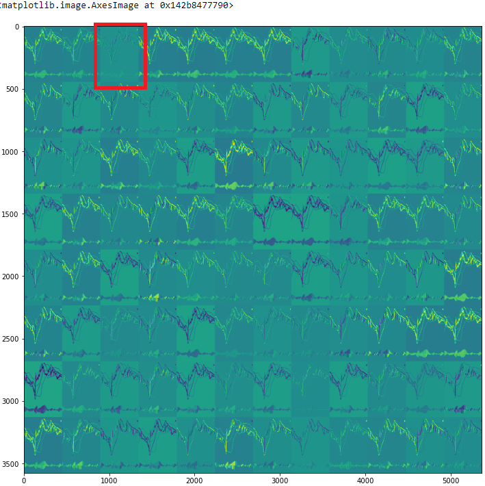
Take a look at the third feature map (2).
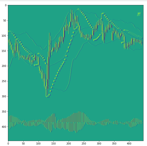
Here the neural network highlights all candlesticks, but with different wicks. Due to this the picture resembles a three-dimensional one. But again, you can see that bearish candlestick wicks and Parabolic have the same color.
Now look at the map 5 of the next convolutional layer (3).
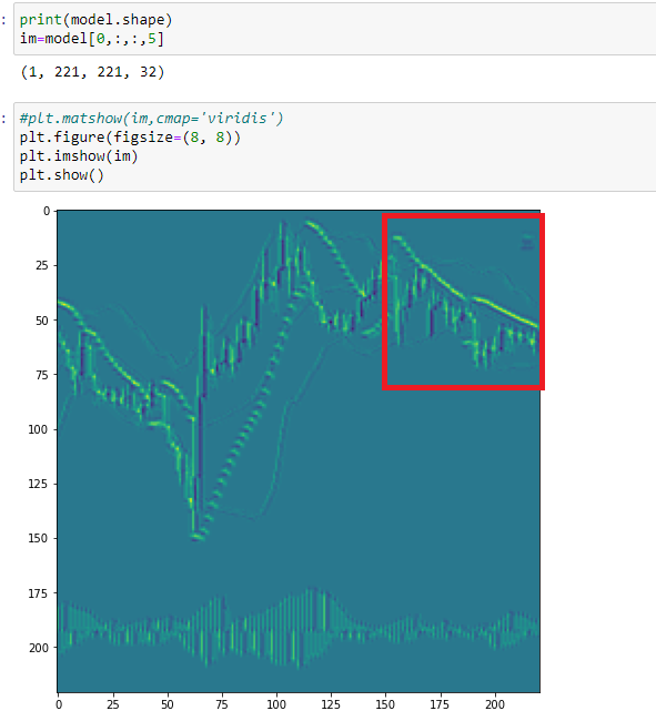
Here, the Parabolic points overlap, and CNN identifies them as a sign of a flat pattern. According to the previous figure, the neural network rendered this section differently. So, we can conclude that the categories of images for training have expanded. We need to introduce one more category to train the neural network - Flat.
Thus, visual examination of Convolutional Neural Network feature maps enables a clearer specification of training tasks. This may also assist in expanding the categories of feature identified by the CNN, as well as in reducing the noise.
Conclusion
Using publicly available tools and capabilities of convolutional neural networks, we can apply an interesting and unconventional approach to technical analysis. And at the same time, this can greatly simplify the preparation of data for neural network training. The visualization of processes occurring inside helps to analyze which input data most affect the quality of training.
In conclusion, I would like to mention optimization. As I wrote before, this was a very simple optimization. However, it should be brought in line with the tasks that we set for our network. In accordance with these tasks, the training array should be divided into categories. Further, these conditions should be used when creating a trading robot.
Translated from Russian by MetaQuotes Ltd.
Original article: https://www.mql5.com/ru/articles/8668
Warning: All rights to these materials are reserved by MetaQuotes Ltd. Copying or reprinting of these materials in whole or in part is prohibited.
This article was written by a user of the site and reflects their personal views. MetaQuotes Ltd is not responsible for the accuracy of the information presented, nor for any consequences resulting from the use of the solutions, strategies or recommendations described.
 Self-adapting algorithm (Part III): Abandoning optimization
 Neural networks made easy (Part 10): Multi-Head Attention
 Multilayer perceptron and backpropagation algorithm
 Developing a self-adapting algorithm (Part II): Improving efficiency
- Free trading apps
- Over 8,000 signals for copying
- Economic news for exploring financial markets
You agree to website policy and terms of use
I'm sorry, but with digital data, it's perverse to process graphics.
Forgive me, but with digital data, processing graphics is a perversion....
1. You have to do everything in png =)
2. For the purposes of neurotrending, reinforcement learning is suitable.... Otherwise you will have to explain to neurons the difference between two graphical images (arrays), and in the presence of digital data this is an unnecessary trick. Neurons understand everything digitally and source data digitally too =)
Well.... I use graphics to identify similarities and then use them as a filter. That's all. I would advise you to also use neurons to analyse text messages...
The point is not to formalise something into "chisels". Zigzag is a problematic indicator in general... Specifically lagging in dynamics and not telling anything....
https://youtu.be/mcQH-OqC0Bs, https://youtu.be/XL5n4X0Jdd8
you're dead wrong on this one. Stop pipsing with the review of one candle and everything will be immediately obvious.
you're dead wrong. Stop pipsing with the review of one candle and everything will be obvious at once.
If we look with the best neural network in our head at the screenshot of the chart, which our artificial neural network is reviewing.... we can see that there's more than one candle on it.
I'm sorry, but with digital data, it's perverse to process graphics.
Forgive me, but with digital data, processing graphics is a perversion....
1. You have to do everything in png =)
2. For the purposes of neurotrending, reinforcement learning is suitable.... Otherwise you will have to explain to neurons the difference between two graphical images (arrays), and in the presence of digital data this is an unnecessary trick. Neurons understand everything digitally and source data digitally too =)
And yes, at the training stage, the hardware resources need to be raised significantly. But this is all within reason.
But at the stage of analysis and response, a neural network needs only an image without additional digitised data. For example, my working neural networks, which analyse time series, are lined up in a chain and each has more than 50 inputs.
So here is the question - where is it better to twist...? At the training stage or at the working stage.