
Developing a multi-currency Expert Advisor (Part 18): Automating group selection considering forward period
Introduction
In Part 7, I considered selection of a group of individual trading strategy instances with the aim of improving the results when they work together. I used two approaches for selection. In the first approach, the group selection took place using the optimization results obtained over the entire optimization time interval. I tried to include in the group those single instances that showed the best results in the optimization interval. In the second approach, a small piece was allocated from the optimization time interval, on which optimization of single instances was not performed. The allocated piece of time interval was then used in the group selection: I tried to include in the group those single instances that showed good (but not the best) results in the optimization interval and at the same time showed approximately the same results in the selected piece of the time interval.
The results were as follows:
- I did not see any clear advantage of selection using the first method over the second method. This may have been due to the short time period of history over which we compared the results of the two methods. Three months is not enough to evaluate a strategy that may have long periods of flat movement.
- The second method showed that on the selected piece of the time interval the results are better if we apply the selection into a group according to the algorithm described in the article for finding single instances of trading strategies with similar results. If we select them simply based on the best possible results over the optimization interval (as in the first method, but only over a shorter interval), then the results of the selected group were noticeably worse.
- It is possible to combine both methods, that is, to construct two groups selected in different ways and then combine the two resulting groups into one.
In Part 13, we implemented automation of the second stage of optimization. Within its framework, single copies of trading strategies obtained in the first stage were selected into a group. We used a simple search using the genetic algorithm of the standard optimizer in the strategy tester. No pre-clustering of single instances (considered in Part 6) have been done. Thus, we automated the selection of groups in the first way. At that time, it was not possible to implement the selection of groups using the second approach, but now is the time to return to this issue. In this article, we will try to achieve the ability to automatically select individual instances of trading strategies into groups, taking into account their behavior in the forward period.
Mapping out the path
As always, let's first look at what we already have and what is missing to solve the problem. We can set the task of optimizing a trading strategy over any required time interval. The words "set a task" should be taken literally: to do this, we create the necessary entries in the tasks table of our database. Accordingly, we can first perform optimization on one time interval (for example, from 2018 to 2022 inclusive), and then on another interval (for example, for 2023).
But with this approach we cannot use the obtained results in the desired way. At each of the two time intervals, optimization will be performed independently, so there will be nothing to compare: the passes of the second optimization will not repeat the passes of the first one in terms of the input parameters' values. The same is true for the genetic optimization we use. It is clear that this is not true for full optimization, but we have never used it and most likely will not use it in the future due to the large number of combinations of optimized parameters.
Therefore, it will be necessary to use the launch of the optimization with the specified forward period. In this case, the tester will use the same combinations of inputs on the forward period as on the main one. But we have not tried running automated optimization with a forward period yet, and we do not know how these results will get into our database. Will we then be able to distinguish between runs in the main period and runs in the forward period? We should check this.
Once we are confident that the database contains all the necessary information about the passes for both the main and forward periods, we can proceed to the next stage. In Part 7, after receiving these results, I manually performed their analysis and selection, using Excel. However, in the context of automation, its use seems inefficient. We try to avoid any manual manipulation of data while obtaining the final EA. Fortunately, all the actions we performed in Excel (recalculating some results, calculating the ratios of pass rates for different testing periods, finding the final score for each strategy group and sorting by it) can be performed in an MQL5 program through SQL queries to our database or running a Python script.
Having sorted by the final assessment, we will take only the topmost group into the final EA. We will perform similar actions for all combinations of selected symbols and timeframes. After normalizing the overall group, including the best groups for all symbol-timeframe pairs, the final EA will be ready.
Let's get started with the implementation, but first let's fix the discovered error.
Fixing a saving error
When I developed the EA to automate the first stage (optimization of single instances of trading strategies), I used only one database. Therefore, there was no question about what database we should receive data from or save data to. In the second stage of optimization, a new auxiliary database was added, which contained the minimum necessary extract from the main database. It was this abbreviated version of the database that was sent to test agents as part of the second stage of optimization.
But due to the approach I had already chosen when implementing a static class for working with the database, I had to use a somewhat inconvenient solution that allows changing the database name if necessary. After changing the name, all subsequent calls to the database connection method used the new name. This is where the error occurred when adding the pass results at the second and third stages. The reason was the lack of switching back to the main base in all the places where it was necessary.
To fix this, I added an additional input to the EA of each stage and to the project auto optimization EA. This input specifies the name of the main database. Apart from fixing the bug, this is also useful because we can better separate the databases used in different articles. For example, in this part, a new main database was used, since we decided to reduce the composition of optimization tasks, but did not want to clear the existing database:
//+------------------------------------------------------------------+
//| Inputs                                                           |
//+------------------------------------------------------------------+
sinput string fileName_   = "database683.sqlite"; // - File with the main database
In the OnInit() function of the second stage EA SimpleVolumesStage2.mq5, inside the LoadParams() function call, a connection was made to an auxiliary database, since the data on the inputs of single instances of trading strategies for joining into a group should be taken from it. After the pass was completed, the OnTester() function was called. In the function, saving the results of the group's passage had to be performed in the main database. But since there was no switch back to the main database, the full results of the pass (48 columns) were attempted to be inserted into a table in the auxiliary database (2 columns).
So we added the missing switch to the main database in the OnInit() function of the second stage EA SimpleVolumesStage2.mq5:
//+------------------------------------------------------------------+
//| Expert initialization function                                   |
//+------------------------------------------------------------------+
int OnInit() {

      ...

// Load strategy parameter sets
   string strategiesParams = LoadParams(indexes);

// Connect to the main database
   DB::Connect(fileName_);
   DB::Close();


     ...

// Create an EA handling virtual positions
   expert = NEW(expertParams);

   if(!expert) return INIT_FAILED;

   return(INIT_SUCCEEDED);
}
In the first and third stage optimization EA, which do not use an auxiliary database, we added the database name taken from the EA's new input to the first call of the database connection method:
DB::Connect(fileName_)
Another type of error I found occurred when, after completion, I wanted to run one of the runs separately. The pass ran and executed normally, but its results were not entered into the database. The reason was that in case of such a launch the task ID remained equal to 0, while in the database, the passes table accepts only a string with the ID of an existing task in the tasks table.
This could be fixed either by making the task ID take the value from the EA inputs (where it is taken from during optimization), or by adding a dummy task with the ID 0 to the database. I ended up choosing the second option so that my single passes launched manually would not be counted as passes performed as part of any specific optimization task. For the added dummy task, it was necessary to specify any ID of an existing process so as not to violate foreign key constraints and the Done status so that this task would not be launched during auto optimization.
After making these corrections, we will return to the main task at hand.
Preparing the code and database
Let's take a copy of the existing database and clear it of data on passes, tasks and jobs. Then we modify the data of the first stage by adding the start date of the forward period. We can remove the second stage from the table of stages. Create one entry in the jobs table for the first stage, specifying the symbol and period (EURGBP H1), as well as the strategy tester parameters. Include optimization only by a single parameter in them so that the number of passes is small. This will allow us to get results faster. For the created job in the tasks table, add one task with a complex optimization criterion.
Launch the project auto optimization EA by specifying the created database in the input parameter. After the first launch, it turned out that the auto optimization EA needed to be improved, since it did not receive information from the database about the necessity to use the forward period. After the additions, the code for the function for obtaining the next optimization task from the database looked like this (the added strings are highlighted in color):
//+------------------------------------------------------------------+
//| Get the next optimization task from the queue                    |
//+------------------------------------------------------------------+
ulong GetNextTask(string &setting) {
// Result
   ulong res = 0;

// Request to get the next optimization task from the queue
   string query = "SELECT s.expert,"
                  "       s.optimization,"
                  "       s.from_date,"
                  "       s.to_date,"
                  "       s.forward_mode,"
                  "       s.forward_date,"
                  "       j.symbol,"
                  "       j.period,"
                  "       j.tester_inputs,"
                  "       t.id_task,"
                  "       t.optimization_criterion"
                  "  FROM tasks t"
                  "       JOIN"
                  "       jobs j ON t.id_job = j.id_job"
                  "       JOIN"
                  "       stages s ON j.id_stage = s.id_stage"
                  " WHERE t.status IN ('Queued', 'Processing')"
                  " ORDER BY s.id_stage, j.id_job, t.status LIMIT 1;";

// Open the database
   if(DB::Connect()) {
      // Execute the request
      int request = DatabasePrepare(DB::Id(), query);

      // If there is no error
      if(request != INVALID_HANDLE) {
         // Data structure for reading a single string of a query result
         struct Row {
            string   expert;
            int      optimization;
            string   from_date;
            string   to_date;
            int      forward_mode;
            string   forward_date;
            string   symbol;
            string   period;
            string   tester_inputs;
            ulong    id_task;
            int      optimization_criterion;
         } row;

         // Read data from the first result string
         if(DatabaseReadBind(request, row)) {
            setting =  StringFormat(
                          "[Tester]\r\n"
                          "Expert=%s\r\n"
                          "Symbol=%s\r\n"
                          "Period=%s\r\n"
                          "Optimization=%d\r\n"
                          "Model=1\r\n"
                          "FromDate=%s\r\n"
                          "ToDate=%s\r\n"
                          "ForwardMode=%d\r\n"
                          "ForwardDate=%s\r\n"
                          "Deposit=10000\r\n"
                          "Currency=USD\r\n"
                          "ProfitInPips=0\r\n"
                          "Leverage=200\r\n"
                          "ExecutionMode=0\r\n"
                          "OptimizationCriterion=%d\r\n"
                          "[TesterInputs]\r\n"
                          "idTask_=%d\r\n"
                          "fileName_=%s\r\n"
                          "%s\r\n",
                          GetProgramPath(row.expert),
                          row.symbol,
                          row.period,
                          row.optimization,
                          row.from_date,
                          row.to_date,
                          row.forward_mode,
                          row.forward_date,
                          row.optimization_criterion,
                          row.id_task,
                          fileName_,
                          row.tester_inputs
                       );
            res = row.id_task;
         } else {
            // Report an error if necessary
            PrintFormat(__FUNCTION__" | ERROR: Reading row for request \n%s\nfailed with code %d",
                        query, GetLastError());
         }
      } else {
         // Report an error if necessary
         PrintFormat(__FUNCTION__" | ERROR: request \n%s\nfailed with code %d", query, GetLastError());
      }

      // Close the database
      DB::Close();
   }

   return res;
}
We also added a function for getting the path to the file of the optimized EA from the current folder relative to the root folder of the terminal EAs:
//+------------------------------------------------------------------+
//| Getting the path to the file of the optimized EA from the current|
//| folders relative to the root folder of terminal EAs              |
//+------------------------------------------------------------------+
string GetProgramPath(string name) {
   string path = MQLInfoString(MQL_PROGRAM_PATH);
   string programName = MQLInfoString(MQL_PROGRAM_NAME) + ".ex5";
   string terminalPath = TerminalInfoString(TERMINAL_DATA_PATH) + "\\MQL5\\Experts\\";
   path =  StringSubstr(path,
                        StringLen(terminalPath),
                        StringLen(path) - (StringLen(terminalPath) + StringLen(programName)));
   return path + name;
}
This allowed the database to specify in the stages table only the file name of the optimized EA without listing the names of the folders it is nested in relative to the root EA folder \MQL5\Experts\.
The following runs of the automatic project optimization EA showed that the results of forward passes were successfully added to the passes table along with the results of regular passes. However, after the stage is completed, it is quite difficult to distinguish which passes belong to which period (main or forward). Of course, we can take advantage of the fact that the forward period passes always come after the regular ones, but this stops working if the results of several optimization problems with a forward period appear in the passes table. So let's add the is_forward column to the passes table to distinguish between regular and forward passes. We will also add the is_optimzation column to make it easy to distinguish between regular passes and passes performed as part of optimization.
Along the way, an inaccuracy was discovered: when forming a SQL query string for inserting data with the results of a pass, we substituted the pass number as a signed integer, using the %d specifier. However, the pass number is an unsigned long integer, so to correctly substitute its value into the string, we should use the %I64u specifier.
Let's add the value of the corresponding function for determining the forward period flag to the code for generating the SQL query for inserting the pass data:
string CTesterHandler::GetInsertQuery(string values, string inputs, ulong pass) {
   return StringFormat("INSERT INTO passes "
                       "VALUES (NULL, %d, %I64u, %d, %s,\n'%s',\n'%s') RETURNING rowid;",
                       s_idTask, pass, (int) MQLInfoInteger(MQL_FORWARD), values, inputs,
                       TimeToString(TimeLocal(), TIME_DATE | TIME_SECONDS));
}
However, it turned out that this would not work as expected. The point is that this function is called from the EA launched in the main terminal in the data frame collection mode. Therefore, the MQLInfoInteger(MQL_FORWARD) call result always returns false for it.
Therefore, the forward period indicator should be obtained in the code that runs on the test agents, and not in the main terminal on the chart, that is, in the test pass completion event handler. An optimization sign has also been added nearby.
//+------------------------------------------------------------------+
//| Handling completion of tester pass for agent                     |
//+------------------------------------------------------------------+
void CTesterHandler::Tester(double custom,   // Custom criteria
                            string params    // Description of EA parameters in the current pass
                           ) {
   ...

// Generate a string with pass data
   data = StringFormat("%d, %d, %s,'%s'",
                       MQLInfoInteger(MQL_OPTIMIZATION),
                       MQLInfoInteger(MQL_FORWARD),
                       data, params);

   ...
}
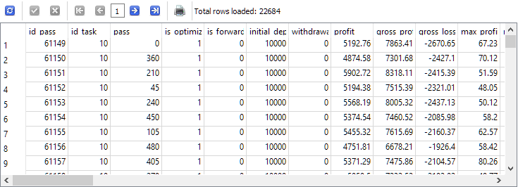
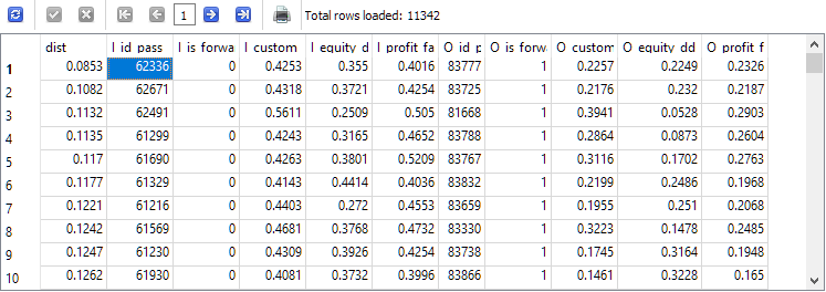
After making these edits and restarting the automatic optimization EA, we finally saw the desired picture in the passes table:
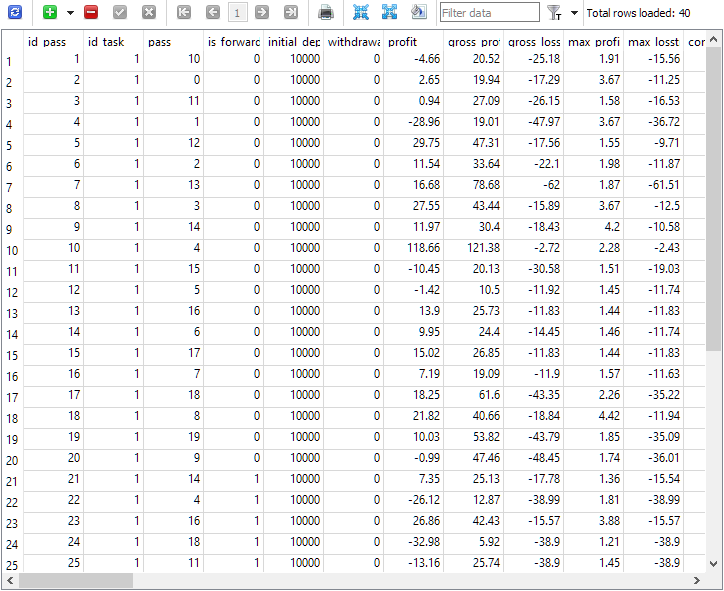
Fig. 1. The passes table after completing the optimization task with a forward period
As can be seen, only 40 passes were performed in the context of the optimization task with id_task = 1. 20 of them were normal (the first 20 strings with is_forward = 0), while the remaining 20 are passes on the forward period (is_forward = 1). Tester pass numbers in the pass column take values from 1 to 20 and each occurs exactly 2 times (once for the main period, the second time for the forward period).
Preparing for full optimization launch
Having verified that the results of passes made using the forward period are now correctly entered into the database, we will conduct a test of the auto optimization that is closer to real conditions. To do this, we will add two stages to the clean database. The first one will optimize a single instance of the trading strategy, but only on one symbol and period (EURGBP H1) over the period from 2018 to 2023. The forward period will not be used at this stage. In the second stage, the group of good single instances obtained in the first stage will be optimized. Now the forward period will already be used: the entire year 2023 is allocated for it.
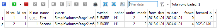
Fig. 2. Stages table with two stages
For each stage in the jobs table, create jobs to be carried out within this stage. In this table, in addition to the symbol and period, the inputs for the optimized EAs with ranges and step changes are indicated.
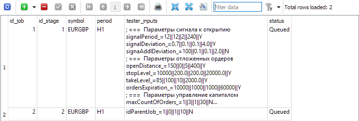
Fig. 3. Jobs table with two jobs for the first and second stages respectively
For the first one (id_job = 1), create several optimization problems that will differ in optimization criterion value (optimization_criterion = 0 ... 7) . Let's go through all the criteria in turn, and use the complex criterion twice: at the beginning and at the end of the first job (optimization_criterion = 7). For the task performed within the second job (id_job = 2), we will use a custom optimization criterion (optimization_criterion = 6)
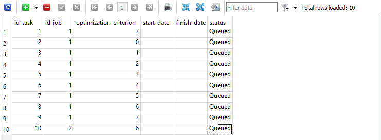
Fig. 4. The tasks table with tasks for the first and second job
Let's launch the auto optimization EA on any terminal chart and wait until all assigned tasks are completed. With the existing agents, the process took about 4 hours in total.
Preliminary analysis of results
In the completed auto optimization, we had only one optimization task that used a forward period. The optimization criterion for it was our custom criterion, which calculated the standardized average annual profit for a given pass. Let's look at the cloud of points with the values of this criterion on the main period.
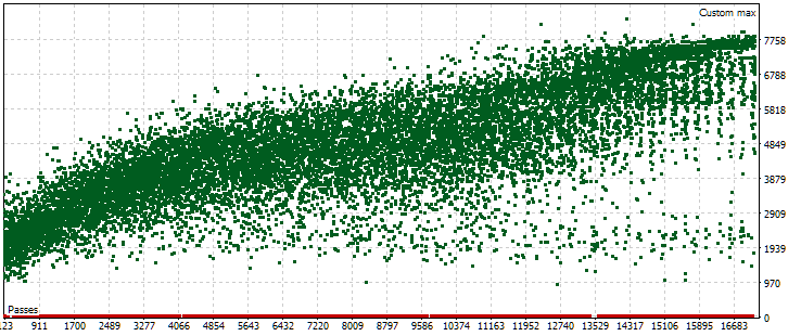
Fig. 5. Cloud of points with values of normalized average annual profit for different passes in the main period
The graph shows that the value of our criterion is in the range from USD 1000 to USD 8000. The red dots corresponding to 0 occur because some combinations of single instance indices in the input parameters result in duplicate values. Such inputs are considered invalid strategy groups and there will be no results from these passes. A general trend towards an increase in the normalized average annual profit in later passes is noticeable. On average, the best results achieved are approximately twice as high as the results of the first passes, in which the parameters are chosen almost randomly.
Now let's look at the point cloud with the results of passes in the forward period. There will be fewer of them (about 13,000 instead of 17,000) due to the combinations of parameters eliminated at the main stage and recognized as incorrect.
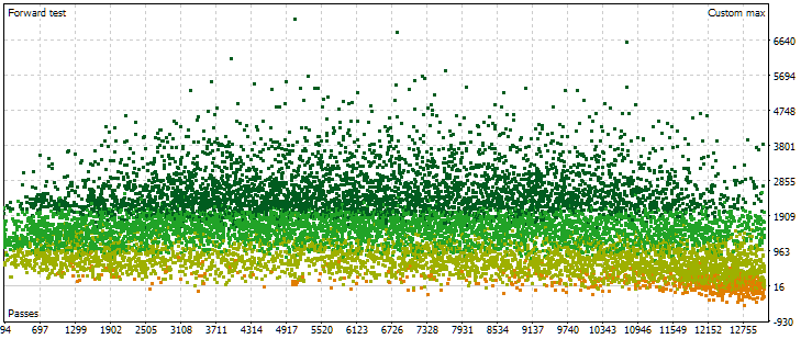
Fig. 6. Cloud of points with values of normalized average annual profit for different passes in the forward period
Here the picture of the points location is already different. There is no significant increase in the results obtained with increasing pass number. On the contrary, we see that as the pass number increases, the results first reach higher values than at the beginning, and then the trend changes to the opposite. With a further increase in the pass number, its results on average begin to decrease, and the rate of decrease increases as we approach the right border of the numbers.
However, as it turns out, this picture will not always be the case. With other settings of the ranges of parameters iterated during optimization, the point clouds for passes on the main and forward periods may look like this:
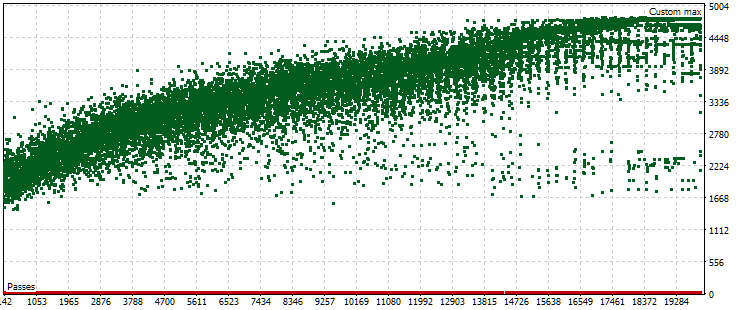
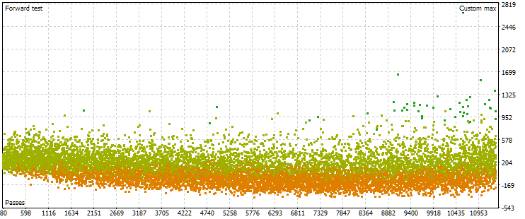
Fig. 7. Cloud of points with values of normalized average annual profit for the main and forward period in case of other optimization settings
As we can see, the picture is approximately the same in the main period, only the criterion range is now slightly different: from USD 1500 to USD 5000. However, in the forward period, the nature of the cloud is completely different. The maximum values are achieved not on the passes that occur approximately in the middle of the optimization, but closer to the end. Also, on average, the criterion values in the forward period are approximately 10 times smaller instead of 3 times, as in the first optimization process.
Intuition suggested that in order to increase the stability of the results obtained over different periods, we need to select a group whose results in the main and forward periods are approximately the same. However, the results obtained made me strongly doubt that we would be able to obtain anything useful this way. Especially in the case when even the maximum value of the criterion in the forward period is noticeably less compared to mediocre values of the criterion in the main period. Let's try anyway. Let's look for conditionally "close" passes in the main and forward periods and look at their results in the main, forward periods and in 2024.
Selecting passes
Let's remember how we chose the best group based on the results in the forward period in Part 7. Here is a summary of the algorithm with minor adjustments:
- Let's adjust the value of the normalized average annual profit for the passes in the forward period, taking for the calculation the maximum drawdown of two values: in the main and forward periods. We get the value of OOS_ForwardResultCorrected.
- In the combined table of optimization results for 2018-2022 (main period) and for 2023 (forward period), calculate the ratio of their values in the main and forward periods for all parameters.
For example, for the number of deals: TradesRatio = OOS_Trades / IS_Trades, while for the normalized average annual profit: ResultRatio = OOS_ForwardResultCorrected / IS_BackResult.
The closer these ratios are to 1, the more identical the values of these indicators are in the two periods. - Let's calculate for all these relations the sum of their deviations from unity. This value will be our measure of the difference between the results of each group in the main and forward periods:
SumDiff = |1 - ResultRatio| + ... + |1 - TradesRatio|. -
Also, take into account that the drawdown could be different for each pass in the main and forward periods. Select the maximum drawdown from two periods and use it to calculate the scaling factor for the sizes of positions opened to achieve the standardized drawdown of 10%:
Scale = 10 / MAX(OOS_EquityDD, IS_EquityDD).
-
Now we want to select the sets where SumDiff is not as prevalent as Scale. To do this, calculate the last parameter:
Res = Scale / SumDiff.
-
Let's sort all groups by the Res value calculated in the previous step in descending order. In this case, the groups, whose results in the main and forward periods were more similar and the drawdown in both periods was smaller, find themselves at the top of the table.
Next, we proposed repeating the selection of groups several times, first removing those that contain the numbers of single copies of trading strategies already included in the selected groups. But this step will be relevant for preliminary clustering of single instances, so that different indices correspond to instances that are dissimilar in results. Since we have not yet reached clustering during auto optimization, we will skip this step.
Instead, we can add a second level of grouping by different timeframes for each symbol and a third level by different symbols.
We will slightly modify the given algorithm. Let's start with the fact that, in essence, we want to understand how far apart two sets of results of the pass are in a space with a dimension equal to the number of compared results (features). To do this, we used the first-order norm with some scaling factor to find the distance from the point with coordinates of the ratios of the compared results from a fixed point with unit coordinates. However, among these relationships, there can be both those close to 1 and those very distant. The latter may unreasonably worsen the overall distance estimate. Therefore, let's try to replace the previously proposed option with the calculation of the usual Euclidean distance between two result vectors, for which we will first apply min-max scaling.
We will need to write a rather complex SQL query in the end (although there may be much more complex queries). Let's take a closer look at the process of creating the required query. We will start with simple queries and gradually make them more complex. We will place some of the results into temporary tables, which will be used in further queries. After each request, we will show what its results look like.
So, the source data from which we need to get something is mainly in the passes table. Let's make sure that they are really there, and immediately select only those passes that were performed within the framework of the required optimization task. In our particular case, the task identifier id_task corresponding to the second stage optimization for EURGBP H1 had the value 10. Therefore, we will use it in the request text:
-- Request 1

SELECT *
  FROM passes p0
 WHERE p0.id_task = 10;
We can see that the entries in the passes table for this task with id_task=10 are present in quantities of more than 22 thousand pieces.
The next step is to combine into one string the results from two lines of this data set, corresponding to the same numbers of tester passes, but different periods: the main and forward periods. We will temporarily limit the number of columns displayed in the result. We will leave only those that can be used to check the validity of the selection of strings. Let's name the resulting columns according to the following rule: add the prefix "I_" to the column name for the main period (In-Sample) and the prefix "O_" for the forward period (Out-Of-Sample):
-- Request 2

SELECT p0.id_pass AS I_id_pass,
       p0.is_forward AS I_is_forward,
       p0.custom_ontester AS I_custom_ontester,
       p1.id_pass AS O_id_pass,
       p1.is_forward AS O_is_forward,
       p1.custom_ontester AS O_custom_ontester
  FROM passes p0
       JOIN
       passes p1 ON p0.pass = p1.pass AND
                    p0.is_forward = 0 AND
                    p1.is_forward = 1
 WHERE p0.id_task = 10 AND p1.id_task = 10
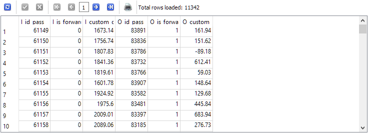
The number of rows as a result was reduced exactly by half, that is, for each pass on the main period in the passes table, there was exactly one pass in the forward period and vice versa.
Now let's return to the first request to perform normalization. If we leave the normalization until later, when we already have separate columns for the same parameter in the main and forward periods, it will be more difficult for us to calculate the minimum and maximum value for both at once. Let's first select a small number of parameters, by which we will evaluate the "distance" between the results in the main and forward periods. For example, let's first practice calculating the distance for three parameters: custom_ontester, equity_dd_relative, profit_factor.
We need to transform the columns with the values of these parameters into columns with values ranging from 0 to 1. Let's use window functions to get the minimum and maximum values for columns within a query. For column names with scaled values, add the prefix "s_" to the original column name. Based on the results returned by this query, we will create and populate a new table using the command
CREATE TABLE ... AS SELECT ... ;
Let's look at the contents of the created and filled new table:
-- Request 3

DROP TABLE IF EXISTS t0;

CREATE TABLE t0 AS
SELECT id_pass,
       pass,
       is_forward,
       custom_ontester,
       (custom_ontester - MIN(custom_ontester) OVER () ) / (MAX(custom_ontester) OVER () - MIN(custom_ontester) OVER () ) AS s_custom_ontester,
       equity_dd_relative,
       (equity_dd_relative - MIN(equity_dd_relative) OVER () ) / (MAX(equity_dd_relative) OVER () - MIN(equity_dd_relative) OVER () ) AS s_equity_dd_relative,
       profit_factor,
       (profit_factor - MIN(profit_factor) OVER () ) / (MAX(profit_factor) OVER () - MIN(profit_factor) OVER () ) AS s_profit_factor
  FROM passes


    WHERE id_task=10;
SELECT * FROM t0;
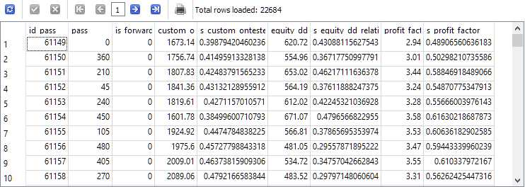
As you can see, next to each estimated parameter, a new column has appeared with the value of this parameter, reduced to the range from 0 to 1.
Now let's reform the text of the second query a little so that it takes data from the new table t0 instead of passes and placed the results into a new table t1. We will take already scaled values and round them for convenience. Let's leave only those strings where the values of normalized profit in the main and forward periods are positive:
-- Request 4

DROP TABLE IF EXISTS t1;

CREATE TABLE t1 AS
SELECT p0.id_pass AS I_id_pass,
       p0.is_forward AS I_is_forward,
       ROUND(p0.s_custom_ontester, 4) AS I_custom_ontester,
       ROUND(p0.s_equity_dd_relative, 4) AS I_equity_dd_relative,
       ROUND(p0.s_profit_factor, 4) AS I_profit_factor,
       p1.id_pass AS O_id_pass,
       p1.is_forward AS O_is_forward,
       ROUND(p1.s_custom_ontester, 4) AS O_custom_ontester,
       ROUND(p1.s_equity_dd_relative, 4) AS O_equity_dd_relative,
       ROUND(p1.s_profit_factor, 4) AS O_profit_factor
  FROM t0 p0
       JOIN
       t0 p1 ON p0.pass = p1.pass AND
                    p0.is_forward = 0 AND
                    p1.is_forward = 1 AND
                    p0.custom_ontester > 0 AND
                    p1.custom_ontester > 0;

SELECT * FROM t1;
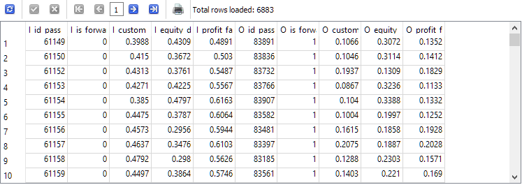
The number of rows has been reduced by about a third compared to the second query, but now we are left with only those runs, in which both the main and forward periods achieved profit.
We have finally reached the final step in the query development process. All that remains is to calculate the distance between the parameter combinations for the main and forward periods in each t1 table row and sort them by increasing distance:
-- Request 5

SELECT
       ROUND(POW((I_custom_ontester - O_custom_ontester), 2) + POW( (I_equity_dd_relative - O_equity_dd_relative), 2) + POW( (I_profit_factor - O_profit_factor), 2), 4) AS dist,
       *
  FROM t1
 ORDER BY dist ASC;
The I_id_pass pass ID from the top string of the obtained results will correspond to the pass with the smallest distance between the values of the results in the main and forward periods.
Let's take it and the ID of the best pass for normalized profit in the main period. They do not match, so we will make a library of parameters for the final EA as described in the previous article. We had to make some minor edits to the files added in the previous article to provide the ability to specify a specific database when creating and exporting a library of parameter sets.
Results
So, we have two settings options in the library. The first one is called "Best for dist(IS, OS) (2018-2023)" — the best optimization pass with the smallest distance between parameter values. The second option is called "Best on IS (2018-2022)" — the best optimization pass for normalized profit in the main period from 2018 to 2022.
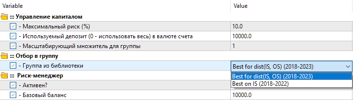
Fig. 8. Selecting a group of settings from the library in the final EA
Let's look at the results of these two groups for the period 2018-2023, which was fully involved in the optimization.
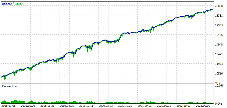
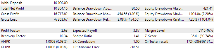
Fig. 9. Results of the first group (best by distance) for the period from 2018 to 2023
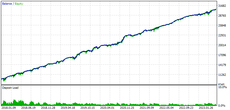
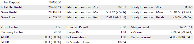
Fig. 10. Results of the second group (the best in terms of profit) for the period from 2018 to 2023
We see that both groups are well normalized over this period of time (the maximum drawdown is USD 1000 in both cases). However, the first one’s average annual profit is approximately two times less than the second one’s (USD 1724 versus USD 3430). The advantages of the first group are not yet visible here.
Let's now look at the results of these two groups for 2024 (before October), which did not participate in the optimization.
Fig. 11. Results of the first group (best by distance) for the period of 2024
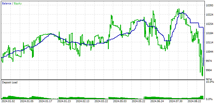
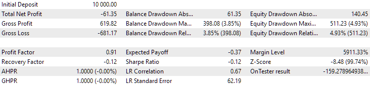
Fig. 12. Results of the second group (best in terms of profit) for the period of 2024
At this point both results are negative, but the second still looks better than the first. It is worth noting that the maximum drawdown during this period was always less than USD 1000.
Since 2024 was not a particularly successful year for this symbol, let's see what the results will be not after, but before the optimization period. Let's take a longer period, since we have such an opportunity (three years from 2015 to 2017).
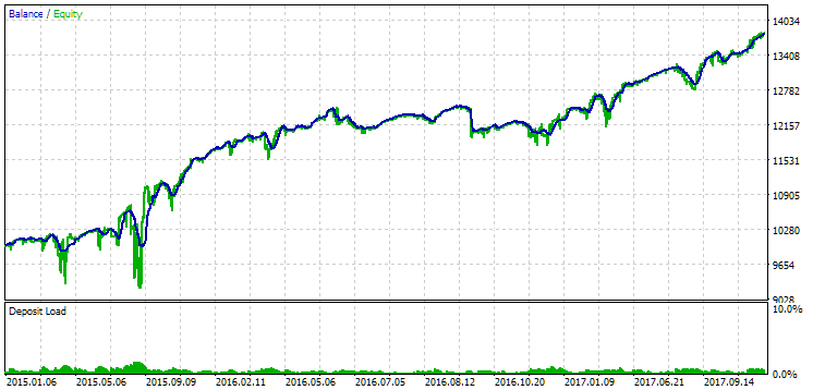
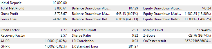
Fig. 13. Results of the first group (best by distance) for the period from 2015 to 2017
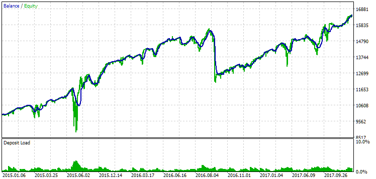
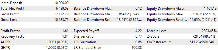
Fig. 14. Results of the second group (best in terms of profit) for the period from 2015 to 2017
During this period, the drawdown has already exceeded the permissible calculated value. In the first version, it was approximately 1.5 times larger, and in the second – approximately 3.5 times larger. In this regard, the first option is somewhat better, since the excess drawdown is noticeably less than in the second and, overall, not very large. Also, in the first version, there is no noticeable dip in the graph in the middle, as in the second version. In other words, the first option showed better adaptability to an unknown period of history compared to the second one. However, in terms of normalized average annual profit, the difference between these two options is not that big (USD 857 versus USD 615). Unfortunately, we cannot calculate this value in advance for an unknown period.
Therefore, during this period, preference will still be on the side of the first option. Let's sum it all up.
Conclusion
We have implemented automation of the second stage of optimization using the forward period. Again, no clear advantages were identified. The task turned out to be much broader and required more time than we initially expected. In the process, many new questions arose that are still waiting for their turn.
We were able to see that if a forward period falls on an unsuccessful period of the EA's work, then we seem not to be able to use it to select good combinations of parameters.
If the duration of the deals is long, the results of the pass with an interruption at the boundary of the main and forward periods may differ significantly from the results of the continuous pass. This also calls into question the advisability of using the forward period in this form - not a forward period in general, but specifically as a way to automatically select parameters that are more likely to show comparable results in the future.
Here we have used one simple way to calculate the distance between the results of the passes. It is possible that making this method more complex will improve the results. We also have not yet started writing an implementation of auto selection of the best pass for inclusion in a group of sets for different symbols and timeframes. Almost everything is ready for the implementation. It will be sufficient to call the SQL queries that we developed from the EA. But since changes will surely still be made to them, we will postpone this automation for the future.
Thank you for your attention! See you soon!
Important warning
All results presented in this article and all previous articles in the series are based only on historical testing data and are not a guarantee of any profit in the future. The work within this project is of a research nature. All published results can be used by anyone at their own risk.
Archive contents
| # | Name | Version | Description | Recent changes |
|---|---|---|---|---|
| MQL5/Experts/Article.15683 | ||||
| 1 | Advisor.mqh | 1.04 | EA base class | Part 10 |
| 2 | Database.mqh | 1.05 | Class for handling the database | Part 18 |
| 3 | database.sqlite.schema.sql | — | Database structure | Part 18 |
| 4 | ExpertHistory.mqh | 1.00 | Class for exporting trade history to file | Part 16 |
| 5 | ExportedGroupsLibrary.mqh | — | Generated file listing strategy group names and the array of their initialization strings | Part 17 |
| 6 | Factorable.mqh | 1.01 | Base class of objects created from a string | Part 10 |
| 7 | GroupsLibrary.mqh | 1.01 | Class for working with a library of selected strategy groups | Part 18 |
| 8 | HistoryReceiverExpert.mq5 | 1.00 | EA for replaying the history of deals with the risk manager | Part 16 |
| 9 | HistoryStrategy.mqh | 1.00 | Class of the trading strategy for replaying the history of deals | Part 16 |
| 10 | Interface.mqh | 1.00 | Basic class for visualizing various objects | Part 4 |
| 11 | LibraryExport.mq5 | 1.01 | EA that saves initialization strings of selected passes from the library to the ExportedGroupsLibrary.mqh file | Part 18 |
| 12 | Macros.mqh | 1.02 | Useful macros for array operations | Part 16 |
| 13 | Money.mqh | 1.01 | Basic money management class | Part 12 |
| 14 | NewBarEvent.mqh | 1.00 | Class for defining a new bar for a specific symbol | Part 8 |
| 15 | Optimization.mq5 | 1.02 | EA managing the launch of optimization tasks | Part 18 |
| 16 | Receiver.mqh | 1.04 | Base class for converting open volumes into market positions | Part 12 |
| 17 | SimpleHistoryReceiverExpert.mq5 | 1.00 | Simplified EA for replaying the history of deals | Part 16 |
| 18 | SimpleVolumesExpert.mq5 | 1.20 | EA for parallel operation of several groups of model strategies. The parameters will be taken from the built-in group library. | Part 17 |
| 19 | SimpleVolumesStage1.mq5 | 1.17 | Trading strategy single instance optimization EA (stage 1) | Part 18 |
| 20 | SimpleVolumesStage2.mq5 | 1.01 | Trading strategies instances group optimization EA (stage 2) | Part 18 |
| 21 | SimpleVolumesStage3.mq5 | 1.01 | The EA that saves a generated standardized group of strategies to a library of groups with a given name. | Part 18 |
| 22 | SimpleVolumesStrategy.mqh | 1.09 | Class of trading strategy using tick volumes | Part 15 |
| 23 | Strategy.mqh | 1.04 | Trading strategy base class | Part 10 |
| 24 | TesterHandler.mqh | 1.04 | Optimization event handling class | Part 18 |
| 25 | VirtualAdvisor.mqh | 1.07 | Class of the EA handling virtual positions (orders) | Part 18 |
| 26 | VirtualChartOrder.mqh | 1.01 | Graphical virtual position class | Part 18 |
| 27 | VirtualFactory.mqh | 1.04 | Object factory class | Part 16 |
| 28 | VirtualHistoryAdvisor.mqh | 1.00 | Trade history replay EA class | Part 16 |
| 29 | VirtualInterface.mqh | 1.00 | EA GUI class | Part 4 |
| 30 | VirtualOrder.mqh | 1.04 | Class of virtual orders and positions | Part 8 |
| 31 | VirtualReceiver.mqh | 1.03 | Class for converting open volumes to market positions (receiver) | Part 12 |
| 32 | VirtualRiskManager.mqh | 1.02 | Risk management class (risk manager) | Part 15 |
| 33 | VirtualStrategy.mqh | 1.05 | Class of a trading strategy with virtual positions | Part 15 |
| 34 | VirtualStrategyGroup.mqh | 1.00 | Class of trading strategies group(s) | Part 11 |
| 35 | VirtualSymbolReceiver.mqh | 1.00 | Symbol receiver class | Part 3 |
Translated from Russian by MetaQuotes Ltd.
Original article: https://www.mql5.com/ru/articles/15683
Warning: All rights to these materials are reserved by MetaQuotes Ltd. Copying or reprinting of these materials in whole or in part is prohibited.
This article was written by a user of the site and reflects their personal views. MetaQuotes Ltd is not responsible for the accuracy of the information presented, nor for any consequences resulting from the use of the solutions, strategies or recommendations described.
- Free trading apps
- Over 8,000 signals for copying
- Economic news for exploring financial markets
You agree to website policy and terms of use
New article Developing multi-currency EA trades (part 18): considering automated group selection for forwards has been published:
By Yuriy Bykov