在线性自回归模型残差上训练非线性 U-Transformer

在现代程序化交易中，开发者普遍面临一个根本性难题：线性模型简单且可解释性强，却无法捕捉金融时序中复杂的非线性关系。而深度神经网络虽然在理论上能够拟合任意非线性关系，但在市场噪声较高、数据量有限的情况下，容易出现过拟合和预测不稳定的问题。

本文提出一套创新的混合方案，通过两阶段建模来化解这一难题：首先，一个基于 25 个特征的线性自回归模型从价格数据中提取关键统计规律；随后，一个专门的 U-Transformer 架构在第一个模型的残差上训练，揭示第一阶段未能捕捉到的隐藏非线性模式。

其核心创新在于对 U-Net 架构（最初为图像分割设计）进行改造，并将 Transformer 模块引入时序分析。该系统使用 MQL5 实现，包含完整的交易逻辑，支持动态持仓管理、参数自动重新优化以及神经网络在线训练。

实验验证表明，混合方案在预测效果上优于纯线性方法，同时保持较高的计算效率与结果可解释性。该系统具备实时运行能力，能够随市场环境变化自动适应。

引言

金融市场属于复杂自适应系统，传统预测方法在此面临几项根本性挑战。第一个也是最明显的挑战就是非线性问题。市场数据中蕴含着复杂、难以用简单线性关系描述的模式：波动率状态切换、对消息的非对称反应，以及级联式流动性效应。然而，将强大的非线性机器学习模型应用于金融数据，往往又会引发第二个问题：过拟合与预测不稳定。

这一问题在程序化交易中尤为突出，因为模型不仅需要精准预测价格走势，还必须在各种市场环境下保持预测的一致性，同时具备足够的计算效率以满足实时运行要求。ARIMA、VAR 等经典计量经济学模型提供了稳定性和可解释性，但其线性本质严重限制了它们建模复杂市场动态的能力。

另一方面，LSTM、GRU、Transformer 等现代深度学习架构理论上足以逼近任意非线性关系，但将它们应用于金融数据时会遇到多重障碍。首先，市场数据中的高噪声会使神经网络记住（拟合）随机波动，而非学习真正有效的模式。其次，金融序列的非平稳性意味着从历史数据中学习到的模式可能很快失效。

第三个问题属于实际工程层面：交易平台的计算资源限制，尤其是在 MQL5 语言环境下，使得开发者难以使用现代深度学习框架。开发者不得不从零实现神经网络算法，这在很大程度上限制了实际可实现架构的复杂度。

本文提出的解决方案基于将预测问题分解为性质不同的两个阶段：线性阶段负责捕捉主要的统计规律，非线性阶段负责建模复杂的残差依赖关系。该方法能够同时发挥两类方法的优势，并将各自的弱点降到最低。

第一阶段的线性自回归模型构建在一个精心设计的 25 维特征空间之上，其中不仅包含经典的价格滞后项，还融入了价格的非线性变换、技术指标以及周期性分量。该模型使用梯度下降进行优化，在具备较高可解释性的同时提供基准级别的预测质量。

第二阶段的神经网络组件采用经过改造的 U-Transformer 架构，它结合了 U-Net 的设计原则（带跳跃连接的编码器 - 解码器结构）与 Transformer 架构的注意力机制。该方法的关键特点在于：神经网络不是在原始价格数据上训练，而是在线性模型的残差上训练，这显著简化了任务并降低了过拟合风险。

这种分解方式天然具备正则化效果：当市场环境发生变化、神经网络组件开始产生不稳定预测时，系统会自动切换至线性模型更稳健的预测结果。这一机制通过自适应加权方案实现，其中神经网络组件的权重取决于两个模型当前的预测质量。

U-Transformer 架构的理论基础

U-Transformer 架构是计算机视觉与自然语言处理两大领域强大概念的融合产物：U-Net 与注意力机制。U-Net 最初是为医学图像分割任务开发的，这类任务要求在保留全局上下文的同时实现精确的目标定位。U-Net 的核心思想是采用对称的编码器 - 解码器结构，并引入横向跳跃连接，使早期网络层提取的细粒度信息能够直接传递到解码器较深层的网络。

在时序分析场景下，这一架构获得了全新的意义。编码器通过提取越来越抽象的模式，逐层压缩时序信息；利用跳跃连接结合抽象表示与细节特征来恢复时间分辨率。这一点对金融数据尤为重要，因为局部波动与全局趋势往往具有同等重要性。

struct UTransformerNet
{
    NeuralLayer encoder_layers[3];     // Encoder: information compression
    NeuralLayer decoder_layers[3];     // Decoder: restore resolution
    AttentionBlock attention_heads[4]; // Multi-head attention
    double skip_connections[3][32];    // U-Net horizontal connections
    double residuals[6000];            // Residuals for training
    double neural_predictions[6000];   // Neural network predictions
};

自注意力机制借鉴自 Transformer 架构，为模型增加了动态聚焦输入序列中最相关部分的能力。与卷积层或循环层不同，注意力机制能够让模型直接建立时间上相隔较远的事件之间的关联，这对金融市场尤为关键，因为事件的影响往往存在滞后性。

void SelfAttention(double &inputs[], AttentionBlock &attention, double &outputs[])
{
    double queries[32], keys[32], values[32];
    
    // Calculate Q, K, V transformations
    for (int i = 0; i < NeuralNodes; i++)
    {
        queries[i] = 0; keys[i] = 0; values[i] = 0;
        for (int j = 0; j < NeuralNodes; j++)
        {
            queries[i] += inputs[j] * attention.query_weights[j][i];
            keys[i] += inputs[j] * attention.key_weights[j][i];
            values[i] += inputs[j] * attention.value_weights[j][i];
        }
    }
    
    // Calculate attention scores: Q × K^T
    for (int i = 0; i < NeuralNodes; i++)
    {
        attention.attention_scores[i] = 0;
        for (int j = 0; j < NeuralNodes; j++)
        {
            attention.attention_scores[i] += queries[i] * keys[j];
        }
        attention.attention_scores[i] /= MathSqrt(NeuralNodes); // Scaling
    }
}

该架构与标准 Transformer 的核心区别在于：它专为一维时间序列做适配，而非标准 Transformer 模型常用的令牌序列表示形式。本模型不使用位置编码，而是采用时间特征（小时数、周期分量），使模型能够考虑交易时段的日内季节性规律。

混合模型：线性回归结合神经网络

这套混合方案的核心思想是将预测结果做加法分解，拆分为两个性质不同的分量：

Final_Prediction = Linear_Model(X) + α × U_Transformer(Residuals)

其中 α 为自适应加权系数，取值取决于两个模型各自的当前预测质量。

线性分量采用拓展特征空间下的经典自回归模型构建：

// Calculate linear prediction
double linear_pred = 0;
for (int i = 0; i < 25; i++)
    linear_pred += g_pair.coeffs[i] * features[i];

神经网络组件不在原始价格数据上训练，而是基于线性模型输出的残差开展训练：

void TrainUTransformer()
{
    // Calculate the residuals of a linear model
    for (int i = 0; i < g_pair.data_size; i++)
    {
        double linear_pred = 0;
        for (int j = 0; j < 25; j++)
            linear_pred += g_pair.coeffs[j] * g_pair.features[i][0][j];
        
        g_pair.neural_net.residuals[i] = g_pair.prices[i] - linear_pred;
    }
    
    // Train a neural network on residuals
    for (int epoch = 0; epoch < NeuralEpochs; epoch++)
    {
        double total_loss = 0;
        for (int i = 0; i < g_pair.data_size; i++)
        {
            double prediction = UTransformerForward(g_pair.coeffs, 
                                                   g_pair.neural_net.residuals[i]);
            double error = prediction - g_pair.neural_net.residuals[i];
            total_loss += error * error;
        }
    }
}

这种分解方式具备几项关键优势。第一，神经网络处理的任务难度大幅降低：建模对象由原始时序变为残差序列。残差通常方差更低，统计平稳性更好，以此简化训练过程，降低过拟合风险。

第二，系统天然实现故障安全机制：一旦神经网络组件输出不稳定预测（损失值偏高），系统会自动提升线性模型分量的权重：

double GetHybridPrediction(double price_t1, double price_t2, double price_t3)
{
    // Linear prediction
    double linear_pred = 0;
    for (int i = 0; i < 25; i++)
        linear_pred += g_pair.coeffs[i] * features[i];
    
    // Neural network correction
    double neural_correction = 0;
    if (g_pair.neural_net.is_trained)
    {
        neural_correction = UTransformerForward(g_pair.coeffs, 0);
    }
    
    // Adaptive weighting
    double confidence = MathMin(g_pair.current_r2, 0.8);
    double neural_weight = g_pair.neural_net.is_trained ? (1.0 - confidence) : 0.0;
    
    return linear_pred + neural_weight * neural_correction;
}

neural_weight 权重系数会随模型质量自动调整：当线性分量 R² 较高（预测效果好）时，分配给神经网络组件的权重就会降低；当 R² 较低时，神经网络获得更高权重。该机制保障系统在各类市场状态下均可稳定运行，避免训练不足的神经网络破坏线性模型高质量的预测结果。

多维特征空间与特征工程

任意机器学习模型的效果，都高度依赖输入特征所含信息量。在金融预测领域，该依赖关系表现得尤为突出——因为市场数据本身具备高噪声、非平稳的特性。本文这套系统采用经过精心设计的 25 维特征空间，既包含传统价格滞后项，也包含其非线性变换结果、技术指标以及周期分量。

基础特征集合包含价格滞后项的一次项与二次项：

void CalculateFeatures(double price_t1, double price_t2, double price_t3, 
                      int bar_index, string symbol, double &features[])
{
    // Linear price components
    features[0] = price_t1;                    // X(t-1)
    features[1] = MathPow(price_t1, 2);        // X(t-1)²
    features[2] = price_t2;                    // X(t-2)
    features[3] = MathPow(price_t2, 2);        // X(t-2)²
    features[4] = price_t3;                    // X(t-3)
    
    // Difference operators (momentum)
    features[5] = (price_t1 - price_t2);      // Short-term momentum
    features[9] = (price_t1 - price_t3);      // Medium-term momentum
    features[18] = MathPow(price_t1 - price_t2, 2); // Quadratic momentum
}

周期分量用于对不同时间尺度下的周期性模式进行建模：

// Low-frequency cycles (daily seasonality)
    features[6] = MathSin(price_t1);
    features[7] = MathCos(price_t1);
    
    // High-frequency cycles (intraday patterns)
    features[13] = MathSin(price_t1 * 1000);
    features[14] = MathCos(price_t1 * 1000);
    
    // Time component (trading session hour)
    datetime bar_time = iTime(symbol, PERIOD_H1, bar_index);
    MqlDateTime dt;
    TimeToStruct(bar_time, dt);
    features[17] = (dt.hour / 24.0);

非线性变换帮助模型适配不同的波动率状态：

// Root and exponential transformations
    features[15] = MathSqrt(MathAbs(price_t1));
    features[16] = MathExp(-MathAbs(price_t1 - price_t2));
    
    // Hyperbolic tangent for limiting outliers
    features[23] = MathTanh(price_t1 - ma);

技术指标补充了有关市场微观结构的信息：

// RSI and its nonlinear versions
    double rsi = 50.0; // Simplified calculation for demonstration
    features[10] = (rsi / 100.0);
    features[21] = MathPow(rsi / 100.0, 2);
    
    // Deviation from the moving average
    double ma = price_t1; // Simplified calculation
    features[11] = (price_t1 - ma);
    
    // Volatility (ATR)
    double atr = MathAbs(price_t1 - price_t2);
    features[12] = atr;
    features[20] = (atr * (price_t1 - price_t2)); // Interaction of volatility and momentum

交互特征作为一个特殊类别，用于建模不同分量之间的非线性效应：

// Pairwise interactions
    features[8] = (price_t1 * price_t2);
    features[19] = (price_t1 / price_t2);
    
    // Triple interactions
    features[22] = (price_t1 * price_t2 * price_t3);
    
    // Constant term
    features[24] = 1.0;

如此丰富多样的特征集合，可让线性模型捕捉范围广泛的市场模式，既包含简单趋势运动，也涵盖复杂非线性形态。而神经网络组件是在这个经过充分特征构建的线性模型的残差之上进行训练，大幅降低了神经网络的学习难度。

MQL5 中的数据结构与内存组织

在 MQL5 环境中实现复杂机器学习算法，需要格外重视内存与数据结构的组织方式。现代深度学习框架会自动管理内存与计算图，与之不同，MQL5 中需要开发者手动设计高效的数据结构。

该系统的核心结构体 PairData，用于存储某一交易对（或货币对）所需的全部数据：

struct PairData
{
    string analyst_symbol;    // Symbol for analysis (EURUSD)
    string trade_symbol;      // Symbol for trading (USDJPY)
    
    // Linear model coefficients
    double coeffs[25];        // Current coefficients
    double best_coeffs[25];   // Best coefficients found
    
    // Quality metrics
    double current_r2;        // Current R²
    double best_r2;           // Best achieved R²
    double learning_rate;     // Adaptive learning rate
    
    // Time series and features
    double prices[6000];                    // Target prices
    double features[6000][50][25];          // Sequences of features
    int data_size;                          // Actual data size
    
    // Position state for averaging/pyramiding
    double last_buy_price;    // Price of the last BUY position
    double last_sell_price;   // Price of the last SELL position
    int buy_levels;           // Number of BUY levels
    int sell_levels;          // Number of SELL levels
    
    // Neural network component
    UTransformerNet neural_net;
};

神经网络层结构体针对矩阵乘法运算做了效率优化：

struct NeuralLayer
{
    double weights[64][64];   // Layer weight matrix
    double biases[64];        // Bias vector
    double outputs[64];       // Neuron outputs
    double gradients[64];     // Gradients for backpropagation
    int size;                 // Actual size of the layer
};

注意力模块实现了简化版的多头注意力机制：

struct AttentionBlock
{
    double query_weights[32][32];  // Query transformation matrix
    double key_weights[32][32];    // Key transformation matrix  
    double value_weights[32][32];  // Value transformation matrix
    double attention_scores[32];   // Attention weights
    double context[32];            // Context vector
};

该内存组织方案的关键特点：采用固定大小的静态数组，而非动态数据结构。这样做是为了实现可预测的内存占用：

// Maximum array sizes are specified as constants
double prices[6000];                    // Maximum 6000 historical points
double features[6000][50][25];          // Sequences of 50 bars
double residuals[6000];                 // Residuals for training the neural network

三维数组 features [6000][50][25] 需要重点说明。第一维对应历史数据样本点；第二维代表长度为 50 的时间序列（供循环网络或注意力机制使用）；第三维为 25 个特征。该存储布局可以为训练与预测提供高效的数据访问能力。

网络权重采用 Xavier/Glorot 初始化方式，保障训练过程稳定：

void InitializeNeuralNetwork()
{
    MathSrand(GetTickCount());
    
    for (int layer = 0; layer < NeuralLayers; layer++)
    {
        int input_size = (layer == 0) ? 25 : NeuralNodes;
        double scale = MathSqrt(2.0 / (input_size + NeuralNodes));
        
        for (int i = 0; i < input_size; i++)
        {
            for (int j = 0; j < NeuralNodes; j++)
            {
                g_pair.neural_net.encoder_layers[layer].weights[i][j] =
                    (MathRand() / 32767.0 - 0.5) * 2.0 * scale;
            }
        }
    }
}

这套内存组织方案，即便在交易平台资源有限的条件下，也可以保障系统高效运行，同时支持复杂机器学习算法的实现。

双组件系统训练算法

混合系统的训练是迭代过程：线性模型组件与神经网络组件交替优化，相互协同。该方式保证收敛稳定，并且让每个组件专门处理预测任务中属于自己的那一部分。

第一步：使用带自适应学习率的梯度下降算法优化线性模型：

void OptimizeCoefficients()
{
    double best_coeffs[25];
    ArrayCopy(best_coeffs, g_pair.coeffs);
    double best_r2 = CalculateR2();
    
    g_pair.learning_rate = InitialLearningRate;
    
    for (int iter = 0; iter < MaxIterations; iter++)
    {
        double gradients[25];
        ArrayInitialize(gradients, 0.0);
        
        // Calculate gradients for all training examples
        for (int i = 0; i < g_pair.data_size; i++)
        {
            double actual = g_pair.prices[i];
            double predicted = 0.0;
            
            // Forward pass of the linear model
            for (int j = 0; j < 25; j++)
                predicted += g_pair.coeffs[j] * g_pair.features[i][0][j];
            
            double error = predicted - actual;
            
            // Accumulate gradients: ∂L/∂w_j = 2 * error * x_j
            for (int j = 0; j < 25; j++)
                gradients[j] += 2.0 * error * g_pair.features[i][0][j];
        }
        
        // Normalize gradients
        for (int j = 0; j < 25; j++)
            gradients[j] /= g_pair.data_size;

梯度裁剪是至关重要的一环，用于防止梯度爆炸：

// Gradient clipping for stability
        double gradient_norm = 0.0;
        for (int j = 0; j < 25; j++)
            gradient_norm += gradients[j] * gradients[j];
        gradient_norm = MathSqrt(gradient_norm);
        
        if (gradient_norm > 1.0)
        {
            for (int j = 0; j < 25; j++)
                gradients[j] /= gradient_norm;
        }
        
        // Update coefficients
        for (int j = 0; j < 25; j++)
            g_pair.coeffs[j] -= g_pair.learning_rate * gradients[j];

自适应学习率会根据优化过程动态自动调整：

double new_r2 = CalculateR2();
        
        if (new_r2 > best_r2)
        {
            // Improvement found - increasing learning rate
            best_r2 = new_r2;
            ArrayCopy(best_coeffs, g_pair.coeffs);
            g_pair.learning_rate *= 1.01;
        }
        else
        {
            // Deterioration - roll back and reduce the rate
            ArrayCopy(g_pair.coeffs, best_coeffs);
            g_pair.learning_rate *= 0.8;
            
            if (g_pair.learning_rate < InitialLearningRate * 0.01)
                break;// Too low speed - stop
        }
    }
}

第二阶段，在已经优化完毕的线性模型的残差数据集上训练神经网络：

void TrainUTransformer()
{
    // Calculate residuals after optimizing a linear model
    for (int i = 0; i < g_pair.data_size; i++)
    {
        double linear_pred = 0;
        for (int j = 0; j < 25; j++)
            linear_pred += g_pair.coeffs[j] * g_pair.features[i][0][j];
        
        g_pair.neural_net.residuals[i] = g_pair.prices[i] - linear_pred;
    }
    
    double best_loss = 1e6;
    int no_improve_count = 0;
    
    for (int epoch = 0; epoch < NeuralEpochs; epoch++)
    {
        double total_loss = 0;
        
        for (int i = 0; i < g_pair.data_size; i++)
        {
            // Forward pass neural networks
            double prediction = UTransformerForward(g_pair.coeffs, 
                                                   g_pair.neural_net.residuals[i]);
            
            // Calculate MSE loss
            double error = prediction - g_pair.neural_net.residuals[i];
            total_loss += error * error;
            
            // Simplified backpropagation (gradient by last layer)
            double gradient = 2.0 * error / g_pair.data_size;
            
            for (int layer = NeuralLayers - 1; layer >= 0; layer--)
            {
                for (int j = 0; j < NeuralNodes; j++)
                {
                    for (int k = 0; k < NeuralNodes; k++)
                    {
                        g_pair.neural_net.encoder_layers[layer].weights[k][j] -=
                            g_pair.neural_net.learning_rate * gradient * 0.01;
                    }
                }
            }
        }
        
        total_loss /= g_pair.data_size;
        
        // Early stopping to prevent overfitting
        if (total_loss < best_loss)
        {
            best_loss = total_loss;
            no_improve_count = 0;
        }
        else
        {
            no_improve_count++;
            if (no_improve_count > 5) break;
        }
    }
}

两个组件学习过程的协同配合，依靠周期性重新优化来实现：

if (g_pair.bars_since_optimization >= OptimizationInterval)
{
    PrepareOptimizationData();
    OptimizeCoefficients();        // Linear model first
    
    // Retrain the neural network every 5 optimization cycles
    if (g_pair.neural_net.training_steps % 5 == 0)
    {
        TrainUTransformer();       // Then the neural network on the new residues
    }
    
    g_pair.bars_since_optimization = 0;
}

U‑Transformer 前向传播流程

U‑Transformer 的前向传播，通过集成注意力机制的编码器‑解码器架构对输入数据做顺序处理。该流程首先构造输入向量，向量内包含时间序列上经过平均处理后的特征：

double UTransformerForward(double &coefficients[], double residual)
{
    double layer_input[32];
    double layer_output[32];
    double attention_output[32];
    
    // Input data preparation: averaging features over a sequence
    double avg_features[25];
    for (int i = 0; i < 25; i++)
    {
        avg_features[i] = 0;
        for (int j = 0; j < 50; j++)
        {
            avg_features[i] += g_pair.features[0][j][i];
        }
        avg_features[i] /= 50;
    }
    
    // Initialize the input layer
    for (int i = 0; i < 25; i++)
        layer_input[i] = avg_features[i];

架构中的编码器部分经由多层依次处理信息，每一层专门负责提取不同抽象层级的特征：

// Pass through encoder layers while preserving skip connections
    for (int layer = 0; layer < NeuralLayers; layer++)
    {
        int input_size = (layer == 0) ? 25 : NeuralNodes;
        
        // Forward pass via a fully connected layer
        ForwardLayer(layer_input, input_size, 
                    g_pair.neural_net.encoder_layers[layer], layer_output);
        
        // Apply self-attention (for the first layers)
        if (layer < TransformerHeads)
        {
            SelfAttention(layer_output, 
                         g_pair.neural_net.attention_heads[layer], 
                         attention_output);
            
            // Residual connection: output = layer + attention
            for (int i = 0; i < NeuralNodes; i++)
                layer_output[i] = layer_output[i] + attention_output[i];
        }
        
        // Save skip connection for decoder
        for (int i = 0; i < NeuralNodes; i++)
            g_pair.neural_net.skip_connections[layer][i] = layer_output[i];
        
        // Prepare the input for the next layer
        for (int i = 0; i < NeuralNodes; i++)
            layer_input[i] = layer_output[i];
    }

全连接层执行带非线性激活的标准线性变换运算：

void ForwardLayer(double &inputs[], int input_size, NeuralLayer &layer, double &outputs[])
{
    for (int j = 0; j < layer.size; j++)
    {
        double sum = layer.biases[j];
        
        // Matrix multiplication: W * x + b
        for (int i = 0; i < input_size; i++)
            sum += inputs[i] * layer.weights[i][j];
        
        // GELU activation for better convergence
        outputs[j] = GELU(sum);
    }
}

GELU（高斯误差线性单元）是 ReLU 的现代替代激活函数：

double GELU(double x) 
{ 
    return 0.5 * x * (1.0 + Tanh(MathSqrt(2.0 / M_PI) * (x + 0.044715 * x * x * x))); 
}

自注意力机制用于计算输入序列不同片段对应的注意力权重：

void SelfAttention(double &inputs[], AttentionBlock &attention, double &outputs[])
{
    double queries[32], keys[32], values[32];
    
    // Calculate Query, Key, Value vectors
    for (int i = 0; i < NeuralNodes; i++)
    {
        queries[i] = 0; keys[i] = 0; values[i] = 0;
        for (int j = 0; j < NeuralNodes; j++)
        {
            queries[i] += inputs[j] * attention.query_weights[j][i];
            keys[i] += inputs[j] * attention.key_weights[j][i];
            values[i] += inputs[j] * attention.value_weights[j][i];
        }
    }
    
    // Softmax normalization of attention weights
    double max_score = attention.attention_scores[0];
    for (int i = 1; i < NeuralNodes; i++)
        if (attention.attention_scores[i] > max_score)
            max_score = attention.attention_scores[i];
    
    double sum_exp = 0;
    for (int i = 0; i < NeuralNodes; i++)
    {
        attention.attention_scores[i] = MathExp(attention.attention_scores[i] - max_score);
        sum_exp += attention.attention_scores[i];
    }
    
    for (int i = 0; i < NeuralNodes; i++)
        attention.attention_scores[i] /= sum_exp;
    
    // Apply attention weights to values
    for (int i = 0; i < NeuralNodes; i++)
    {
        outputs[i] = 0;
        for (int j = 0; j < NeuralNodes; j++)
            outputs[i] += attention.attention_scores[j] * values[j];
    }
}

最终聚合环节采用平均池化，输出一个标量结果：

// Decoder part (simplified - uses only the last encoder output)
    double final_sum = 0;
    for (int i = 0; i < NeuralNodes; i++)
        final_sum += layer_output[i];
    
    return final_sum / NeuralNodes; // Average pooling
}

该架构实现多层次信息处理：底层网络提取局部模式，注意力机制对长距离依赖关系建模，跳跃连接为最终预测保留细节信息。

交易信号生成系统

这套混合系统的交易信号生成采用双层架构，根据信号质量在不同信号源间自动切换。该架构使系统能够适应多种多样的市场环境，避免其中一个模型效果恶化后整体性能随之下降。

主要信号源是 U‑Transformer，当模型训练质量达标后启用：

void ProcessPair()
{
    // Obtain data for analysis from the analyst symbol
    double price_t1 = iClose(g_pair.analyst_symbol, PERIOD_H1, 1);
    double price_t2 = iClose(g_pair.analyst_symbol, PERIOD_H1, 2);
    double price_t3 = iClose(g_pair.analyst_symbol, PERIOD_H1, 3);
    
    // Current price of the trading symbol
    double current_ask = SymbolInfoDouble(g_pair.trade_symbol, SYMBOL_ASK);
    double current_bid = SymbolInfoDouble(g_pair.trade_symbol, SYMBOL_BID);
    double current_price = (current_ask + current_bid) / 2.0;
    
    int signal = 0;
    
    // MAIN SIGNAL: U-Transformer (at high quality)
    if (g_pair.neural_net.is_trained && g_pair.neural_net.loss < 0.01)
    {
        double features[25];
        CalculateFeatures(price_t1, price_t2, price_t3, 1, g_pair.analyst_symbol, features);
        double neural_prediction = UTransformerForward(g_pair.coeffs, 0);
        
        double neural_threshold = 0.0001;
        
        if (neural_prediction > neural_threshold) signal = 1;      // BUY signal
        else if (neural_prediction < -neural_threshold) signal = -1; // SELL signal
    }
}

当神经网络尚未完成训练，或是输出结果不理想时，就会启用备用信号源：

// BACKUP SIGNAL: Linear Model
    if (signal == 0 && g_pair.current_r2 > 0.1)
    {
        double predicted_price = GetHybridPrediction(price_t1, price_t2, price_t3);
        double base_threshold = g_pair.current_r2 * 0.001;
        
        if (predicted_price > current_ask + base_threshold) signal = 1;
        if (predicted_price < current_bid - base_threshold) signal = -1;
    }

自适应响应阈值是关键设计，阈值大小会跟随模型质量做缩放。神经网络信号使用固定阈值，因为该模型是在归一化残差数据集上完成训练。线性模型信号的阈值与模型 R² 成正比；拟合效果越好，系统可以生成越激进的交易信号。

记录信号来源，保证交易决策过程透明、可追溯：

if (OpenPosition(true, lot))
{
    Print(g_pair.trade_symbol, ": BUY opened by ",
          g_pair.neural_net.is_trained ? "U-TRANSFORMER" : "LINEAR",
          " R2=", DoubleToString(g_pair.current_r2, 3),
          " UT_Loss=", DoubleToString(g_pair.neural_net.loss, 6));
}

将分析品种与交易品种分离开，支持基于合成图表（例如 Renko 砖形图）进行交易。举个例子，可以基于 EURUSD 的 Renko 砖形 K 线做分析，生成信号用来交易 EURUSD。该方式拓展了系统能力，借助额外信息有机会进一步提升信号质量。

仓位管理策略与风险控制

仓位管理系统实现两套互补策略：加仓摊平亏损仓位、金字塔加仓放大盈利仓位。这两套策略可以自动适配市场行情，并与信号生成系统深度集成。

仓位跟踪结构体包含实现复杂策略所需要的全部参数：

struct PairData
{
    // Track the status of positions
    double last_buy_price;      // Price of the last BUY position
    double last_sell_price;     // Price of the last SELL position
    int buy_levels;             // Number of BUY position levels
    int sell_levels;            // Number of levels of SELL positions
    bool last_was_averaging;    // Flag of the last averaging operation
};

当价格相对于已开持仓反向移动指定点数，且系统持续输出同方向信号时，摊平加仓策略将会被触发：

// AVERAGING BUY positions
if (g_pair.last_buy_price > 0)
{
    double distance_points = (g_pair.last_buy_price - current_price) / 
                            SymbolInfoDouble(g_pair.trade_symbol, SYMBOL_POINT);
    
    if (EnableAveraging && distance_points >= DistancePoints && signal == 1 &&
        g_pair.buy_levels < MaxAveragingLevels)
    {
        double lot = NormalizeLot(g_pair.trade_symbol, LotSize * AveragingLotMultiplier);
        if (OpenPosition(true, lot))
        {
            g_pair.last_buy_price = current_price;
            g_pair.buy_levels++;
            g_pair.last_was_averaging = true;
            
            Print(g_pair.trade_symbol, ": BUY AVERAGING level ", g_pair.buy_levels,
                  " at distance ", DoubleToString(distance_points, 1), " points");
        }
    }
}

金字塔加仓策略逻辑与之相反，它针对盈利持仓进行加仓：

// PYRAMIDING BUY positions
distance_points = (current_price - g_pair.last_buy_price) / 
                  SymbolInfoDouble(g_pair.trade_symbol, SYMBOL_POINT);

if (EnablePyramiding && distance_points >= DistancePoints && signal == 1 &&
    g_pair.buy_levels < MaxPyramidingLevels && !g_pair.last_was_averaging)
{
    double lot = NormalizeLot(g_pair.trade_symbol, LotSize * PyramidingLotMultiplier);
    if (OpenPosition(true, lot))
    {
        g_pair.last_buy_price = current_price;
        g_pair.buy_levels++;
        
        Print(g_pair.trade_symbol, ": BUY PYRAMIDING level ", g_pair.buy_levels,
              " at distance ", DoubleToString(distance_points, 1), " points");
    }
}

该实现的一项关键特性：禁止摊平加仓与金字塔加仓同时启用（依靠 last_was_averaging 标志位），避免策略演变成无序的反复加仓。

交易量管理针对不同操作类型使用对应的乘数系数：

double NormalizeLot(string symbol, double lot)
{
    double min_lot = SymbolInfoDouble(symbol, SYMBOL_VOLUME_MIN);
    double max_lot = SymbolInfoDouble(symbol, SYMBOL_VOLUME_MAX);
    double lot_step = SymbolInfoDouble(symbol, SYMBOL_VOLUME_STEP);
    
    lot = MathRound(lot / lot_step) * lot_step;
    lot = MathMax(min_lot, MathMin(max_lot, lot));
    
    return lot;
}

这套仓位管理架构，在管控最大风险的同时赋予仓位操作灵活性。系统可适应不同市场环境，在某些情形下使用摊平策略，在另一些情形下采用金字塔加仓，并配有明确的止盈规则。

模型系数自动重新优化

能够适应不断变化的市场环境，是所有交易系统的核心要求。金融市场具备非平稳特性，宏观经济事件、市场微观结构改变、市场参与者行为转变，都会造成统计模式发生变化。本系统实现自动重新优化，基于滑动历史数据窗口周期性更新模型参数。

当累计生成指定数量的新 K 线时，触发重优化流程：

void OnTick()
{
    if (!g_initialized) return;
    
    ProcessPair();
    
    // Check the need for reoptimization
    if (isNewBar())
    {
        if (g_pair.bars_since_optimization >= OptimizationInterval)
        {
            PrepareOptimizationData();      // Data preparation
            OptimizeCoefficients();         // Re-optimization of the linear model
            
            // Retrain the neural network every 5 cycles
            if (g_pair.neural_net.training_steps % 5 == 0)
            {
                TrainUTransformer();
            }
            
            g_pair.bars_since_optimization = 0;
        }
    }
}

优化阶段的数据准备采用固定大小的滑动窗口，以此在模型稳定性与环境适应性之间取得平衡。

void PrepareOptimizationData()
{
    g_pair.data_size = 0;
    
    int available_bars = iBars(g_pair.analyst_symbol, PERIOD_H1);
    if (available_bars < 50)
    {
        Print("WARNING: Insufficient bars for ", g_pair.analyst_symbol);
        return;
    }
    
    int max_data_points = MathMin(OptimizationBars, 6000);
    
    for (int i = 50; i < MathMin(max_data_points + 50, available_bars - 1); i++)
    {
        if (g_pair.data_size >= 6000) break;
        
        double price_t0 = iClose(g_pair.analyst_symbol, PERIOD_H1, i - 1);
        if (price_t0 <= 0) continue;
        
        g_pair.prices[g_pair.data_size] = price_t0;
        
        // Collection of time sequences of features
        for (int j = 0; j < 50; j++)
        {
            double price_t1 = iClose(g_pair.analyst_symbol, PERIOD_H1, i - j);
            double price_t2 = iClose(g_pair.analyst_symbol, PERIOD_H1, i - j - 1);
            double price_t3 = iClose(g_pair.analyst_symbol, PERIOD_H1, i - j - 2);
            
            if (price_t1 <= 0 || price_t2 <= 0 || price_t3 <= 0) continue;
            
            double features[25];
            CalculateFeatures(price_t1, price_t2, price_t3, i - j, 
                            g_pair.analyst_symbol, features);
            
            for (int k = 0; k < 25; k++)
            {
                g_pair.features[g_pair.data_size][j][k] = features[k];
            }
        }
        
        g_pair.data_size++;
    }
    
    Print(g_pair.analyst_symbol, ": Prepared ", g_pair.data_size, " data points");
}

优化流程内置了最优系数存储机制，系统会持续监测模型拟合效果：

void OptimizeCoefficients()
{
    if (g_pair.data_size < 10)
    {
        Print(g_pair.analyst_symbol, ": Insufficient data (", g_pair.data_size, ")");
        return;
    }
    
    double best_coeffs[25];
    ArrayCopy(best_coeffs, g_pair.coeffs);
    double best_r2 = CalculateR2();
    
    // Improvement criterion for continuing optimization
    double initial_r2 = g_pair.current_r2;
    
    for (int iter = 0; iter < MaxIterations; iter++)
    {
        // ... gradient descent code ...
        
        double new_r2 = CalculateR2();
        
        if (new_r2 > best_r2)
        {
            best_r2 = new_r2;
            ArrayCopy(best_coeffs, g_pair.coeffs);
            g_pair.learning_rate *= 1.01; // Acceleration when improving
        }
        else
        {
            ArrayCopy(g_pair.coeffs, best_coeffs);
            g_pair.learning_rate *= 0.8;  // Slowdown when deteriorating
            
            if (g_pair.learning_rate < InitialLearningRate * 0.01)
                break;
        }
        
        // Stop criterion for minimum improvement
        if (iter > 10 && (best_r2 - initial_r2) < MinR2Improvement)
            break;
    }
    
    // Update the best coefficients
    ArrayCopy(g_pair.coeffs, best_coeffs);
    g_pair.current_r2 = best_r2;
    
    if (best_r2 > g_pair.best_r2)
    {
        g_pair.best_r2 = best_r2;
        ArrayCopy(g_pair.best_coeffs, best_coeffs);
    }
    
    Print(g_pair.analyst_symbol, ": R2=", DoubleToString(g_pair.current_r2, 4),
          " Best=", DoubleToString(g_pair.best_r2, 4));
}

其中 R² 指标用于评估模型质量，它表示模型可解释的方差占比：

double CalculateR2()
{
    if (g_pair.data_size < 10) return 0.0;
    
    double sum_actual = 0.0;
    double sum_squared_total = 0.0;
    double sum_squared_residual = 0.0;
    
    // Calculate the average value
    for (int i = 0; i < g_pair.data_size; i++)
        sum_actual += g_pair.prices[i];
    double mean_actual = sum_actual / g_pair.data_size;
    
    // Calculate R² components
    for (int i = 0; i < g_pair.data_size; i++)
    {
        double actual = g_pair.prices[i];
        double predicted = 0.0;
        
        for (int j = 0; j < 25; j++)
            predicted += g_pair.coeffs[j] * g_pair.features[i][0][j];
        
        double residual = actual - predicted;
        double total_variance = actual - mean_actual;
        
        sum_squared_residual += residual * residual;
        sum_squared_total += total_variance * total_variance;
    }
    
    if (sum_squared_total <= 0.0) return 0.0;
    
    return 1.0 - (sum_squared_residual / sum_squared_total);
}

基于残差的神经网络在线训练

相比线性优化，神经网络模块的在线训练是一项更为复杂的任务。神经网络不会在每个优化周期都重新训练，而是每 5 个优化周期训练一次。该设计既可以防止过拟合，也能够降低计算开销。

void TrainUTransformer()
{
    if (g_pair.data_size < 10)
    {
        Print("Insufficient data for U-Transformer training: ", g_pair.data_size);
        return;
    }
    
    // Calculate residuals from the optimized linear model
    for (int i = 0; i < g_pair.data_size; i++)
    {
        double linear_pred = 0;
        for (int j = 0; j < 25; j++)
            linear_pred += g_pair.coeffs[j] * g_pair.features[i][0][j];
        
        g_pair.neural_net.residuals[i] = g_pair.prices[i] - linear_pred;
    }
    
    Print("Training U-Transformer on ", g_pair.data_size, " residuals...");
    
    double best_loss = 1e6;
    int no_improve_count = 0;

该训练流程使用适配 MQL5 平台限制的简化版反向传播算法：

for (int epoch = 0; epoch < NeuralEpochs; epoch++)
    {
        double total_loss = 0;
        
        for (int i = 0; i < g_pair.data_size; i++)
        {
            // Forward pass
            double prediction = UTransformerForward(g_pair.coeffs, 
                                                   g_pair.neural_net.residuals[i]);
            g_pair.neural_net.neural_predictions[i] = prediction;
            
            // Calculate MSE loss
            double error = prediction - g_pair.neural_net.residuals[i];
            total_loss += error * error;
            
            // Simplified backpropagation
            double gradient = 2.0 * error / g_pair.data_size;
            
            // Update weights (simplified scheme)
            for (int layer = NeuralLayers - 1; layer >= 0; layer--)
            {
                for (int j = 0; j < NeuralNodes; j++)
                {
                    for (int k = 0; k < NeuralNodes; k++)
                    {
                        g_pair.neural_net.encoder_layers[layer].weights[k][j] -=
                            g_pair.neural_net.learning_rate * gradient * 0.01;
                    }
                }
            }
        }
        
        total_loss /= g_pair.data_size;
        
        // Early stopping mechanism
        if (total_loss < best_loss)
        {
            best_loss = total_loss;
            no_improve_count = 0;
        }
        else
        {
            no_improve_count++;
            if (no_improve_count > 5) break; // Stop if there are no improvements
        }
        
        if (epoch % 5 == 0)
            Print("U-Transformer epoch ", epoch, " loss: ", DoubleToString(total_loss, 6));
    }

训练收尾阶段会更新神经网络的各项指标与运行状态：

g_pair.neural_net.loss = best_loss;
    g_pair.neural_net.is_trained = true;
    g_pair.neural_net.training_steps++;
    
    Print("U-Transformer training completed. Loss: ", DoubleToString(best_loss, 6));
}

神经网络质量判定条件（损失值小于 0.01），决定系统何时可以信任神经网络信号：

// In the signal generation function
if (g_pair.neural_net.is_trained && g_pair.neural_net.loss < 0.01)
{
    // Use U-Transformer to generate signals
    double neural_prediction = UTransformerForward(g_pair.coeffs, 0);
    // ...
}

这套在线学习架构，使神经网络模块能够适配不断变化的市场环境，同时兼顾计算效率，抑制过拟合现象。

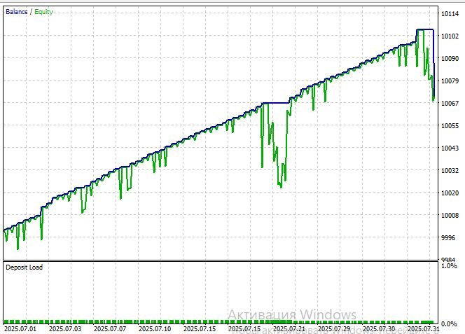
本文 EA 以回归模型相关文章中的 EA 程序为基础，在此之上新增了这套混合模型。 

我们在 EURUSD 的 M15 时间周期上测试模型表现，测试起始时间为 2025 年 7 月 1 日：

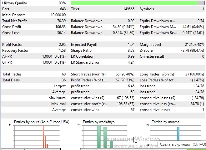
测试得到的夏普比率表现相当可观：

结论

本文提出的混合系统证明：在 MQL5 交易平台的约束条件下，将现代深度学习架构与传统计量经济学方法相结合具备现实可行性。把预测问题拆解为线性、非线性两个阶段，能够充分发挥两类方法各自优势，同时尽可能规避二者的短板。

本工作的主要成果包括：将 U‑Net 架构成功适配用于金融时间序列分析；引入注意力机制对长距离依赖关系进行建模；实现多信号源自动切换系统。依靠模块自适应权重分配与参数周期性重优化，系统可以在各类市场环境下稳定运行。

该方案的实际价值在于可直接用于实盘交易。系统内置完整交易逻辑，包含仓位管理、风险管控以及详尽的交易日志输出。分析品种与交易品种相互分离，拓展了跨市场相关性策略的应用空间。

但也需要客观承认当前实现方案存在的局限性。简化版反向传播算法、缺少现代正则化手段、固定不变的网络结构，限制了神经网络模块的性能上限。代码使用静态数组而非动态数据结构，给系统的可扩展性带来很大制约。

即便如此，本文提出的思路为交易系统开发开辟了极具潜力的研究方向。基于线性模型残差训练神经网络这一设计思想，不只局限于金融市场，还可以推广到更多预测类问题。系统采用模块化架构，便于开展各类实验，可替换测试不同神经网络以及仓位管理策略。

本文尤为重要的一点启示：即便是 MQL5 这类开发环境受限的平台，同样可以实现高阶机器学习算法。这为广大无法使用主流深度学习框架的交易者与开发者创造了更多可能性。

参考

• 《Attention Is All You Need》（Vaswani 等人，2017）
• 《U‑Net：用于生物医学图像分割的卷积网络》（Ronneberger 等人，2015）