
Portfolio trading in MetaTrader 4

Magnus
ab integro saeclorum nascitur ordo
Publius
Vergilius Maro, Eclogues
Introduction
The portfolio principle is known from long ago. By diversifying the funds in several directions, investors create their portfolios reducing the overall loss risk and making income growth more smooth. The portfolio theory has gained momentum in 1950 when the first portfolio mathematical model has been proposed by Harry Markowitz. In 1980s, a research team from Morgan Stanley has developed the first spread trading strategy paving the way for the group of market neutral strategies. The present-day portfolio theory is diverse and complex making it almost impossible to describe all portfolio strategies in a single article. Therefore, only a small range of speculative strategies along with their possible implementation in MetaTrader 4 platform will be considered here.
Some definitions applied in this article are as follows:
- Portfolio (basket, synthetic instrument) — set of positions at multiple trading instruments with calculated optimal volumes. Positions remain open for some time, are tracked as one and closed with a common financial result.
- Portfolio (basket, synthetic instrument) adjustment — changing the set of portfolio instruments and/or their volumes to minimize losses or fix intermediate results.
- Synthetic volume — number of synthetic positions (number of times the portfolio was bought or sold).
- Virtual profit/loss — financial result that can be obtained when holding a position within a certain time interval.
Classic investment portfolios are usually applied at stock markets. However, such an approach does not suit Forex much since most portfolios are speculative here. They are created and traded slightly differently. As far as Forex is concerned, the portfolio trading is actually a multi-currency trading, however, not all multi-currency strategies are portfolio ones. If symbols are traded independently and no total result dynamics is tracked, this is a multi-symbol trading. If several independent systems trade on a single trading account, this is a strategy portfolio. Here we will consider a portfolio trading in the narrow sense — when a synthetic position is formed out of several symbols and is managed afterwards.
Principles
Portfolio development consists of the two stages: selecting symbols and calculating lots and directions for them. Here we will discuss only a few simple portfolio development methods along with algorithm samples. In particular, we propose the ordinary least squares method (OLS) and principal component analysis (PCA) as a basis. More information can be found here:
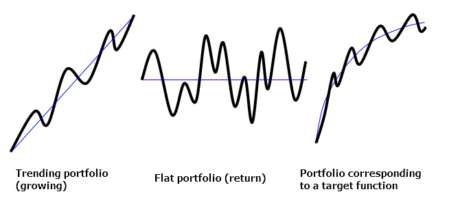
When developing a portfolio, it is usually necessary to define the desired portfolio graph behavior. Portfolio graph represents the changes of the total profit of all positions included into the portfolio within a certain time interval. Portfolio optimization is a search for a combination of lots and directions best fitting the desired portfolio behavior. For example, depending on our task, it may be necessary for a portfolio to have a recurrence to the average value or attributes of a clearly marked trend or its chart should be similar to a chart of a function.
Three portfolio types (trend, flat, function):
A portfolio can be represented by the following equation:
A*k1 + B*k2 + C*k3 + ... = F,
where
A, B, C ... are time series corresponding to portfolio symbols
k1, k2, k3 ... are symbol lots (positive — buy, negative — sell)
F — target function (set by values in time series points)
This is a multivariate linear regression equation with a zero constant term. Its roots can be easily found using OLS. First of all, time series should be made comparable meaning that price points should be brought to a deposit currency. In this case, each element of each timeseries will represent a virtual profit value of a single lot of the appropriate symbol at a particular time. Preliminary price logarithmation or using price differences are usually recommended in statistical application tasks. However, that may be unnecessary and even harmful in our case since critical overall symbols dynamics data would be destroyed along the way.
The target function defines the portfolio graph type. The target function values should be preliminarily calculated in each point accordingly. For example, when developing a simple growing portfolio (trend portfolio), the target portfolio will have the values 0, 1*S, 2*S, 3*S, etc., where S is an increment — the money value, to which the portfolio should be increased at each bar on a predetermined interval. The OLS algorithm adds A, B, C, ... time series so that their total sum is looking to repeat the target function chart. To achieve this, the OLS algorithm minimizes the sum of squared deviations between the series sum and the target function. This is a standard statistical task. No detailed understanding of the algorithm operation is required since you can use a ready-made library.
It may also happen that the target function contains only zero values (flat portfolio). In this case, an additional ratio sum limit should be added (for example: k1 + k2 + k3 + ... = 1) to bypass solving a regression equation with zero roots. The alternative is to move an equation term to the right making it a target function receiving the ratio of -1, while the remaining terms are optimized as usual. In this case, we equate the basket of instruments to a selected instrument, thus creating a spread portfolio. Finally, the more advanced PCA algorithm can be used to develop such portfolios. It applies the instrument covariance matrix to calculate the coefficient vector corresponding to the point cloud cross section hyperplane with the portfolio's minimum residual variance. Again, you do not need to understand the algorithm in details here since you can use a ready-made library.
Algorithms
Now, it is time to implement all the ideas described above using MQL language. We will use a well-known ALGLIB math library adapted for MT4. Sometimes, issues may arise during its installation, so I will dwell more on it. If several terminals are installed on a PC, it is very important to find the correct data folder since the compiler does not see the library if it is located in another terminal's data folder.
Installing ALGLIB library:
- download the library (https://www.mql5.com/en/code/11077), unpack zip file;
- open 'include' folder and find Math directory inside;
- launch the МetaТrader 4 platform, to which the library should be added;
- select the menu command: File — Open Data Folder;
- open MQL4 and Include subfolder;
- copy Math folder to Include folder of the terminal;
- check the results: *.mhq files should be inside MQL4\Include\Math\Alglib.
The sample function calculating the contract price is shown below:
double ContractValue(string symbol,datetime time,int period)
  {
   double value=MarketInfo(symbol,MODE_LOTSIZE);                     // receive lot size
   string quote=SymbolInfoString(symbol,SYMBOL_CURRENCY_PROFIT);     // receive calculation currency

   if(quote!="USD")                                                  // if the calculation currency is not USD, perform conversion
     {
      string direct=FX_prefix+quote+"USD"+FX_postfix;                // form a direct quote for calculation currency
      if(MarketInfo(direct,MODE_POINT)!=0)                           // check if it exists
        {
         int shift=iBarShift(direct,period,time);                    // find the bar by time
         double price=iClose(direct,period,shift);                   // receive the bar's quote
         if(price>0) value*=price;                                   // calculate the price
        }
      else
        {
         string indirect=FX_prefix+"USD"+quote+FX_postfix;           // form a reverse quote for the calculation currency
         int shift=iBarShift(indirect,period,time);                  // find the bar by time
         double price=iClose(indirect,period,shift);                 // receive the bar's quote
         if(price>0) value/=price;                                   // calculate the price
        }
     }

   if(Chart_Currency!="USD")                                         // if the target currency is not USD, perform a conversion
     {
      string direct=FX_prefix+Chart_Currency+"USD"+FX_postfix;       // form a direct quote for the target currency
      if(MarketInfo(direct,MODE_POINT)!=0)                           // check if it exists
        {
         int shift=iBarShift(direct,period,time);                    // find the bar by time
         double price=iClose(direct,period,shift);                   // receive the bar's quote
         if(price>0) value/=price;                                   // calculate the price
       }
      else
        {
         string indirect=FX_prefix+"USD"+Chart_Currency+FX_postfix;  // form a reverse quote for the target currency
         int shift=iBarShift(indirect,period,time);                  // find the bar by time
         double price=iClose(indirect,period,shift);                 // receive the bar's quote
         if(price>0) value*=price;                                   // calculate the price
        }
     }

   return(value);
  }
This function will always be used in the future. It works with currency pairs, indices, futures and CFDs. Besides, it also considers symbol prefixes and postfixes (FX_prefix, FX_postfix) applied by some brokers. The result is converted into a target currency (Chart_Currency). If we multiply the returned function value by the current symbol price, we obtain the price of the symbol's one lot. After summing all contract prices in the portfolio considering lots, we obtain the price of the entire portfolio. If we multiply the function value by a price difference in time, we receive profit or loss generated during that price change.
The next step is calculating the virtual profit for all individual lot contracts. The calculation is implemented as a two-dimensional array where the first dimension is a point index in the calculated interval, while the second dimension is a symbol index (the second dimension size can be limited by a certain number knowing that the amount of symbols in the portfolio will obviously not exceed it):
double EQUITY[][100]; // first dimension is for bars, while the second one is for symbols
First, we should store initial prices for all symbols (on the left boundary of the calculated interval). Then, the difference between the initial and final prices is calculated at each point of the calculatied interval and multiplied by the contract price. Each time, we shift to the right by one time interval in the loop:
   for(int i=0; i<variables+constants; i++)                              // portfolio symbols loop (variable and model constants)
     {
      int shift=iBarShift(SYMBOLS[i],Timeframe,zero_time);               // receive bar index by time for a zero point
      opening[i]=iClose(SYMBOLS[i],Timeframe,shift);                     // receive the bar's price and save it in the array
     }

   points=0;                                                             // calculate points in the variable
   datetime current_time=zero_time;                                      // start a loop from the zero point
   while(current_time<=limit_time)                                       // pass along the time labels in the optimization interval
     {
      bool skip_bar=false;
      for(int i=0; i<variables+constants; i++)                           // portfolio symbol loop (variables and model constants)
         if(iBarShift(SYMBOLS[i],Timeframe,current_time,true)==-1)       // check bar existence for the symbol
            skip_bar=true;                                               // if the bar does not exist, skip it for other symbols
      if(!skip_bar)                                                      // continue operation if the bar is synchronized between all symbols
        {
         points++;                                                       // increase the number of points by one
         TIMES[points-1]=current_time;                                   // store time label in memory
         for(int i=0; i<variables+constants; i++)                        // main profit calculation loop for all symbols in the point
           {
            int shift=iBarShift(SYMBOLS[i],Timeframe,current_time);      // receive the bar index by time
            closing[i]=iClose(SYMBOLS[i],Timeframe,shift);               // receive the bar's price
            double CV=ContractValue(SYMBOLS[i],current_time,Timeframe);  // calculate the contract price
            profit[i]=(closing[i]-opening[i])*CV;                        // calculate profit by price difference and cost
            EQUITY[points-1,i]=profit[i];                                // save the profit value
           }
        }
      current_time+=Timeframe*60;                                        // shift to the next time interval
     }
In the above code fragment, zero_time — time of the calculated interval's left boundary, limit_time — time of the calculated interval's right boundary, Timeframe — number of minutes in one bar of the working timeframe, points — total number of detected points in the calculated interval. The time label strict compliance rule is used in the example above. If a bar for a certain time label is absent even at one symbol, a position is skipped and a shift is made to the next one. Managing time labels is very important for preliminary data preparation, since data misalignment on different symbols may cause serious distortions in the portfolio.
The sample portfolio data for three symbols and an independent function (square root parabola):
DATE/TIME AUDJPY GBPUSD EURCAD MODEL 03.08.16 14:00 0 0 0 0 03.08.16 15:00 -61,34 -155 -230,06 10,21 03.08.16 16:00 -82,04 -433 -219,12 14,43 03.08.16 17:00 -39,5 -335 -356,68 17,68 03.08.16 18:00 147,05 -230 -516,15 20,41 03.08.16 19:00 169,73 -278 -567,1 22,82 03.08.16 20:00 -14,81 -400 -703,02 25 03.08.16 21:00 -109,76 -405 -753,15 27 03.08.16 22:00 -21,74 -409 -796,49 28,87 03.08.16 23:00 51,37 -323 -812,04 30,62 04.08.16 00:00 45,43 -367 -753,36 32,27 04.08.16 01:00 86,88 -274 -807,34 33,85 04.08.16 02:00 130,26 -288 -761,16 35,36 04.08.16 03:00 321,92 -194 -1018,51 36,8 04.08.16 04:00 148,58 -205 -927,15 38,19 04.08.16 05:00 187 -133 -824,26 39,53 04.08.16 06:00 243,08 -249 -918,82 40,82 04.08.16 07:00 325,85 -270 -910,46 42,08 04.08.16 08:00 460,02 -476 -907,67 43,3 04.08.16 09:00 341,7 -671 -840,46 44,49
Now that we have prepared data, it is time to send them to the optimization model. The optimization is to be performed using LRBuildZ, LSFitLinearC and PCABuildBasis functions from ALGLIB library. These functions are briefly described inside the library itself, as well as the official project website: http://www.alglib.net/dataanalysis/linearregression.php and here: http://www.alglib.net/dataanalysis/principalcomponentsanalysis.php.
First, make sure to include the library:
#include <Math\Alglib\alglib.mqh>
Next, the code fragment considering the model features should be set for each optimization model. First, let's examine the sample trend model:
   if(Model_Type==trend)
     {
      int info,i,j;                                                                                  // define working variables
      CLinearModelShell LM;                                                                          // define a special object model
      CLRReportShell AR;                                                                             // define a special object report
      CLSFitReportShell report;                                                                      // define yet another object
      CMatrixDouble MATRIX(points,variables+1);                                                      // define a matrix for storing all data
      if(Model_Growth==0) { Alert("Zero model growth!"); error=true; return; }                       // verify the model parameters
      for(j=0; j<points; j++)                                                                        // calculate the target function by optimization interval points
        {
         double x=(double)j/(points-1)-Model_Phase;                                                  // calculate the X coordinate
         if(Model_Absolute) x=MathAbs(x);                                                            // make the model symmetrical if necessary
         MODEL[j]=Model_Growth*x;                                                                    // calculate the Y coordinate
        }
      double zero_shift=-MODEL[0]; if(zero_shift!=0) for(j=0; j<points; j++) MODEL[j]+=zero_shift;   // shift the model vertically to the zero point
      for(i=0; i<variables; i++) for(j=0; j<points; j++) MATRIX[j].Set(i,EQUITY[j,i]);               // download the symbol data to the matrix
      for(j=0; j<points; j++) MATRIX[j].Set(variables,MODEL[j]);                                     // download the model data to the matrix
      CAlglib::LRBuildZ(MATRIX,points,variables,info,LM,AR);                                         // launch the regression calculation
      if(info<0) { Alert("Error in regression model!"); error=true; return; }                        // check the result
      CAlglib::LRUnpack(LM,ROOTS,variables);                                                         // receive equation roots
     }
At first, this may seem complicated, but basically everything is simple. At the start, the linear trend function is calculated and its values are placed to the MODEL array. The Model_Growth parameter sets the growth value for the entire calculation interval (the value, by which the portfolio should grow in the deposit currency). Model_Absolute and Model_Phase parameters are optional and are of no importance at the current stage. The matrix is created for calculations (MATRIX). Data on the virtual profit of all contracts from EQUITY array, as well as the target function values from MODEL array are downloaded to the last row of the matrix. The number of independent regression equation variables is stored in 'variables'. LRBuildZ function is called afterwards to perform calculation. After that, the regression equation roots are written to ROOTS array using LRUnpack function. All complex math is located inside the library, while you can use the ready-made functions. The main difficulty is of technical nature here and related to setting all calls correctly and preserving the data during the preparations.
The same code fragment can be used for any function. Simply replace MODEL array contents with your target function. Sample square root parabolic function calculation is shown below:
      for(j=0; j<points; j++)                               // calculate the target function by optimization interval points
        {
         double x=(double)j/(points-1)-Model_Phase;         // calculate the X axis value
         int sign=(int)MathSign(x);                         // define the value sign
         if(Model_Absolute) sign=1;                         // make the model symmetrical if necessary
         MODEL[j]=sign*Model_Growth*MathSqrt(MathAbs(x));   // calculate the Y axis value
        }
Below is an example of a more complex function representing the sum of a linear trend and harmonic oscillations:
      for(j=0; j<points; j++)                                     // calculate the target function by optimization interval points
        {
         double x=(double)j/(points-1)*Model_Cycles-Model_Phase;  // calculate the X axis value
         if(Model_Absolute) x=MathAbs(x);                         // make the model symmetrical if necessary
         MODEL[j]=Model_Amplitude*MathSin(2*M_PI*x);              // calculate the Y axis value
        }
In the example above, it is possible to manage a trend size (using Model_Growth parameter) and oscillation amplitude (using Model_Amplitude parameter). Number of oscillation cycles is set by Model_Cycles, while oscillation phase shift is performed using Model_Phase.
Additionally, the vertical shift should be performed to let the function be equal to zero at a zero point to ensure the calculations are correct:
   double zero_shift=-MODEL[0];   // read the model value at the zero point
   if(zero_shift!=0)              // make sure it is not zero
      for(j=0; j<points; j++)     // pass along all interval points
         MODEL[j]+=zero_shift;    // shift all model points
These examples make it easy to develop a custom function. You can create any function type depending on your task and trading setup. The more complex the function type, the more difficult it is to select the best solution, since the market is not obliged to follow the function. Here, the function is only an approximation.
You do not need a target function to create spread and return flat portfolios. For example, if you want to create a spread between two symbol baskets, the optimized basket is downloaded to the main part of the matrix, while the reference basket is used as a target function and downloaded to the last column of the matrix as a total amount:
   for(i=0; i<variables; i++)                    // cycle by the optimized basket symbols
      for(j=0; j<points; j++)                    // cycle by the calculated interval points
         MATRIX[j].Set(i,EQUITY[j,i]);           // upload symbol values of the optimized basket to the matrix columns
   for(i=variables; i<variables+constants; i++)  // cycle by the reference basket symbols
      for(j=0; j<points; j++)                    // cycle by the calculated interval points
         MODEL[j]+=EQUITY[j,i]*LOTS[i];          // upload symbol values of the reference basket to the matrix last column
Below is a sample flat portfolio calculation where LSFitLinearC function makes the portfolio as symmetrical as possible around zero within the calculated interval:
   if(Model_Type==fitting)
     {
      int info,i,j;                                                                        // define working variables
      CLSFitReportShell report;                                                            // define the special object model
      CMatrixDouble CONSTRAIN(1,variables+1);                                              // define the matrix of linear limitations
      CMatrixDouble MATRIX(points,variables);                                              // define the matrix for storing all data
      ArrayInitialize(MODEL,0);                                                            // fill the model with zeros
      CONSTRAIN[0].Set(variables,1);                                                       // set the only limitation
      for(i=0; i<variables; i++) CONSTRAIN[0].Set(i,1);                                    // sum of roots should be equal to one
      for(i=0; i<variables; i++) for(j=0; j<points; j++) MATRIX[j].Set(i,EQUITY[j,i]);     // download symbol data to the matrix
      CAlglib::LSFitLinearC(MODEL,MATRIX,CONSTRAIN,points,variables,1,info,ROOTS,report);  // calculate the optimization model using OLS
      if(info<0) { Alert("Error in linear fitting model!"); error=true; return; }          // check the result
     }
Below is yet another important example of calculating a flat portfolio with the minimum variance using PCA method. Here, PCABuildBasis function calculates the ratios so that the portfolio graph remains as compressed within the calculation interval as possible:
   if(Model_Type==principal)
     {
      int info,i,j;                                                                        // define working variables
      double VAR[];                                                                        // define the variance array
      ArrayResize(VAR,variables);                                                          // convert the array to the necessary dimension
      CMatrixDouble VECTOR(variables,variables);                                           // define the coefficient vector matrix
      CMatrixDouble MATRIX(points,variables);                                              // define the matrix for storing all data
      for(i=0; i<variables; i++) for(j=0; j<points; j++) MATRIX[j].Set(i,EQUITY[j,i]);     // upload symbol data to the matrix
      CAlglib::PCABuildBasis(MATRIX,points,variables,info,VAR,VECTOR);                     // calculate the orthogonal basis using PCA
      if(info<0) { Alert("Error in principal component model!"); error=true; return; }     // check the result
      for(i=0; i<variables; i++) ROOTS[i]=VECTOR[i][variables-1];                          // upload optimal ratios
     }
If you feel overwhelmed by all these math concepts, do not worry. As I have already said, you do not need to understand all the mathematical details to develop and use portfolios. Generally, the sequence of stages looks as follows:
| 1 | Calculating virtual profit for portfolio symbols with single lots |
| 2 | Calculating the target function values |
| 3 | Lot optimization algorithm |
| 4 | Portfolio volume normalization |
| 5 | Graph calculation and trading using the portfolio |
Now that we have obtained ROOTS array of optimal ratios using a number of procedures, it is time to turn the ratios into lots. To do this, we need normalization: scaling and rounding. Setting a required scale makes lots convenient to trade. Rounding is necessary to bring the lots capacity in line with broker requirements. Sometimes, it is recommended to perform normalization by portfolio total margin, but this method has serious drawbacks (since the margin of individual symbols varies and can change). Therefore, it is much more reasonable to perform normalization by a portfolio price or its volatility.
Below is a simple example of the normalization algorithm by the portfolio price:
      double total_value=0;                                                                         // define the variable for the portfolio price
      for(int i=0; i<variables+constants; i++)                                                      // pass along all portfolio symbols
         total_value+=closing[i]*ContractValue(SYMBOLS[i],limit_time,Timeframe)*MathAbs(LOTS[i]);   // calculate and sum the price components

      if(total_value==0) { Alert("Zero portfolio value!"); error=true; return; }                    // make sure the result is not zero
      scale_volume=Portfolio_Value/total_value;                                                     // find a scaling ratio

      for(int i=0; i<variables+constants; i++)                                                      // pass along all portfolio symbols again
         LOTS[i]=NormalizeDouble(LOTS[i]*scale_volume,Lots_Digits);                                 // convert the lots to the required total price
Here, the portfolio price is equated to the required one via the proportions. Portfolio_Value — required portfolio price, total_value — total portfolio price with the default ratios, scale_volume — scaling ratio, Lots_Digits — lot capacity, LOTS — array of the lot values suitable for trading.
Lot values form the final portfolio structure. Positive lots correspond to a long position, while negative lots — to a short one. Knowing the portfolio structure, we can plot its chart and perform trading operations with the portfolio. Below is a sample portfolio structure after normalization:
| Symbol | AUDJPY | GBPUSD | EURCAD |
| Lot | -0,07 | -0,11 | -0,11 |
The portfolio graph is plotted only by Close prices and displayed in a separate indicator subwindow. In order to build the portfolio graph, we need to calculate each chart bar the same way virtual profits for separate symbols have been previously calculated. However, now they are summarized considering assigned lots:
   for(int j=draw_begin; j>=draw_end; j--)                                                   // cycle by chart bars within the drawing interval
     {
      double profit=0;                                                                       // start with the value
      for(int i=0; i<variables; i++)                                                         // pass along all symbols
        {
         if(Fast_Period>0 && Slow_Period>0 && number!=N_TOTAL)                               // perform auxiliary checks
           {
            int shift=iBarShift(SYMBOLS[i],Period(),Time[j]);                                // obtain bar index by time
            double CV=ContractValue(SYMBOLS[i],Time[j],Period());                            // calculate the contract price
            double fast=iMA(SYMBOLS[i],Period(),Fast_Period,0,MODE_SMA,PRICE_CLOSE,shift);   // calculate the slow average
            double slow=iMA(SYMBOLS[i],Period(),Slow_Period,0,MODE_SMA,PRICE_CLOSE,shift);   // calculate the fast average
            profit+=(fast-slow)*CV*LOTS[i];                                                  // calculate the oscillation model
           }
         else
           {
            int shift=iBarShift(SYMBOLS[i],Period(),Time[j]);                                // receive the bar index by time
            double closing=iClose(SYMBOLS[i],Period(),shift);                                // receive the symbol price in the point
            double CV=ContractValue(SYMBOLS[i],Time[j],Period());                            // calculate the contract price
            profit+=(closing-OPENINGS[i])*CV*LOTS[i];                                        // calculate profit by price difference and cost
           }
        }
      BUFFERS[number].buffer[j]=NormalizeDouble(profit,2);                                   // save the profit value in the indicator array
     }
In this code fragment, we can see that the chart is plotted between the initial and final bars: draw_begin and draw_end. The portfolio value is equal to the sum of profits/losses at all symbols calculated as a price difference multiplied by a contract price and previously calculated lot. I have skipped technical aspects related to indicator buffers, formatting and the like. The sample ready-made portfolio indicator is described in the section below.
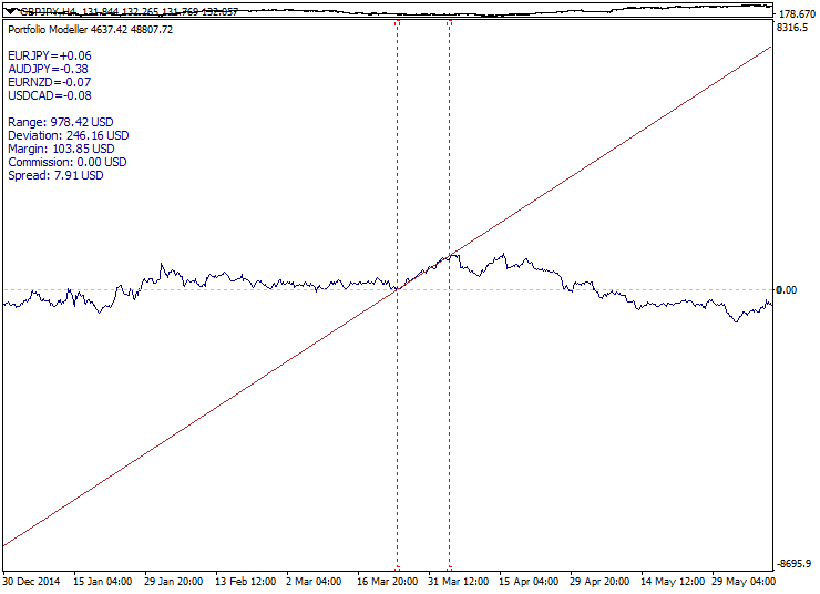
Here you can examine the sample portfolio graph construction (indicator bottom subwindow) with the target function graph attached:
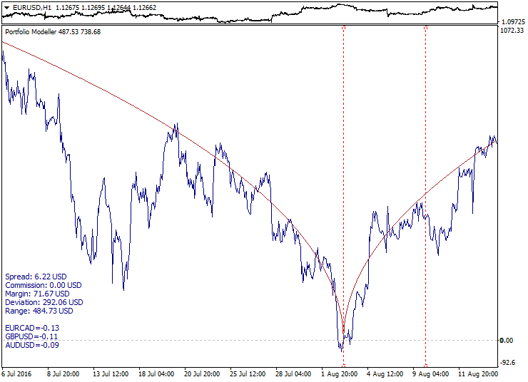
Here, the square root parabola made symmetrical relative to the reference point (Model_Absolute=true) is used as the target function. Calculated interval boundaries are shown as red dotted lines, while the portfolio graph tends to move along the target function line both in and out of the calculated interval.
You can perform technical analysis of portfolio graphs similar to ordinary symbol price charts, including applying moving averages, trend lines and levels. This extends analytical and trading capabilities allowing you to select the portfolio structure for forming a certain trading setup on a portfolio graph, for example correction after a trend impulse, trend weakening, exiting a flat, overbought-oversold, convergence-divergence, breakout, level consolidation and other setups. Trading setup quality is affected by portfolio composition, optimization method, target function and selected history segment.
It is necessary to know the portfolio's volatility to select an appropriate trading volume. Since the portfolio chart is initially based on a deposit currency, you can assess a portfolio fluctuation range and potential drawdown depth directly in that currency using the "crosshair" cursor mode and "pulling".
A trading system should be based on portfolio behavior properties and setup statistics. Until now, we have not mentioned the fact that the portfolio behavior may change dramatically outside the optimization interval. A flat may turn into a trend, while a trend may turn into a reversal. A trading system should also consider that the portfolio properties are prone to change over time. This issue will be discussed below.
Trading operations with a portfolio comprise of a one-time buying/selling all portfolio symbols with calculated volumes. For more convenience, it would be reasonable to have a special Expert Advisor to perform all the routine work, including obtaining portfolio structure data, preparing synthetic positions, tracking entry levels, fixing profit and limiting losses. We will apply the following terms concerning the EA operation: long synthetic portfolio position and short synthetic portfolio position (where long positions are replaced with short ones and vice versa). The EA should be able to accumulate positions, track synthetic volumes, as well as perform portfolio netting and transformation. The sample EA is considered in the next section, though its structure is not explained due to the article volume constraints.
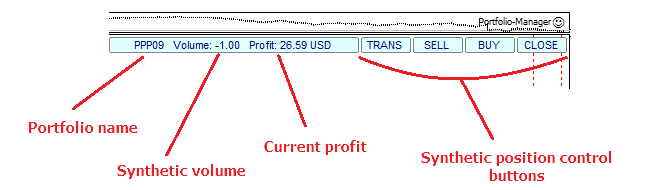
Below is the sample minimalistic interface for a portfolio EA:
Sometimes, it is necessary to build not one but several portfolios. In the simplest case, it is needed for comparing two portfolios. Some tasks require an entire portfolio series to be built on a single history segment resulting in a set of portfolios containing certain patterns. In order to implement such tasks, the algorithm generating portfolios according to a certain template is required. The example of implementing such an indicator can be found in the next section. Here, we are going to describe only its most critical operation features.
We need to arrange a structure array to store the data of multiple portfolios, for example:
struct MASSIVE                     // define the structure containing multiple data types
  {
   string symbol[MAX_SYMBOLS];     // text array for the portfolio symbols
   double lot[MAX_SYMBOLS];        // numerical array for lots
   string formula;                 // string with the portfolio equation
   double direction;               // portfolio direction attribute
   double filter;                  // filter attribute
  };

MASSIVE PORTFOLIOS[DIM_SIZE];      // create the structure array for the group of portfolios
In this code fragment, DIM_SIZE sets the maximum size for storing portfolios. The structure is organized the following way: symbol — portfolio symbol array, lot — lot array for portfolio symbols, formula — text string with the portfolio equation, direction — portfolio direction (long or short), filter — filter attribute (included/excluded). Applying the structure array is more convenient and reasonable than using separate arrays.
The structure array can also be created for storing portfolio graph buffer arrays:
struct STREAM{double buffer[];};     // define the structure containing a numerical array
STREAM BUFFERS[DIM_SIZE];            // create the structure array
Portfolios within the set vary by their symbol combinations. These combinations may be defined in advance or generated according to certain rules. Working with a set of portfolios may include several stages depending on a task. Let's consider the following sequence of stages here:
| 1 | Calculating charts of separate portfolios |
| 2 | Combining a set of portfolios at a zero point |
| 3 | Reversing portfolios relative to a zero level |
| 4 | Applying the filter to a set of portfolios |
| 5 | Summarization — forming a superportfolio |
The image below illustrates these steps:
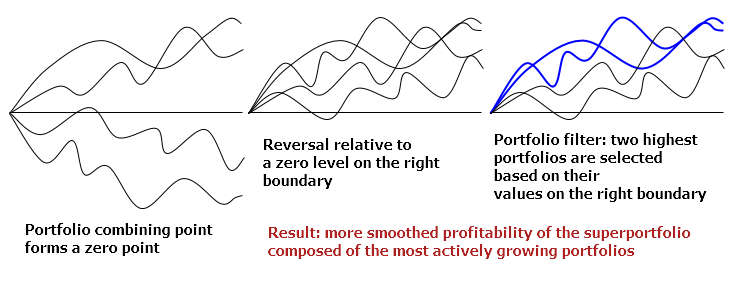
A vertical shift is used to combine portfolios. Portfolio is reversed when multiplied by -1. Finally, a filter is applied by sorting and sampling by values. No detailed description of these algorithms is provided here to avoid a huge bulk of routine code.
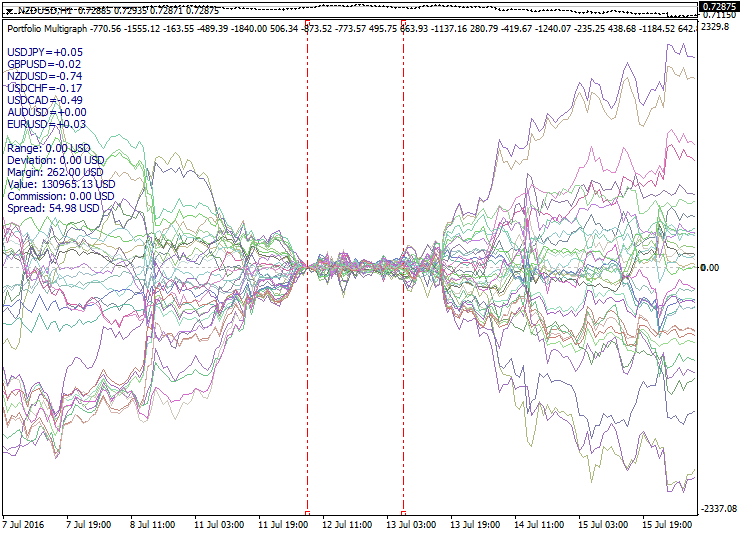
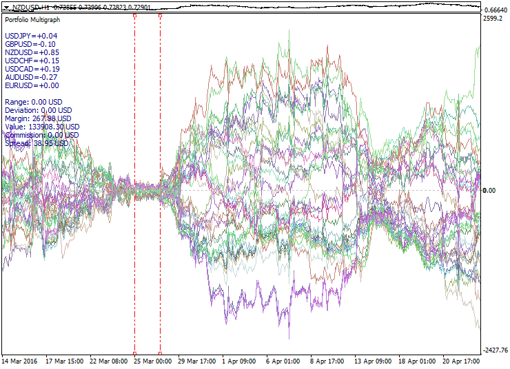
Below is a sample set of portfolios constructed following the mentioned principles:
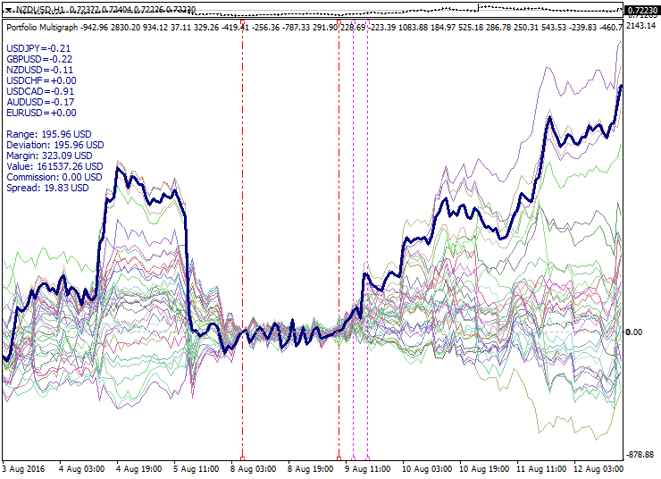
The graph shows a set of portfolios calculated by PCA model with a short period. The calculated interval boundaries are shown as the red dashed lines. Here we can see the expansion of the portfolio set on either side of the optimization interval. The zero point is selected at the left optimization interval boundary, while the moments of reversal relative to zero and the filter application are marked by the purple dotted lines. The thick line outlines the superportfolio consisting of the most active portfolios and thereby having a decent run from the zero point.
Combining portfolios provides additional possibilities for analysis and developing trading strategies, for example diversification between portfolios, spreads between portfolios, convergence-divergence of the set of portfolios, waiting for twisting of a portfolio set, moving from one portfolio to another and other approaches.
Implementation examples
The methods described in the current article have been implemented as a portfolio indicator and a semi-automated EA. Here you can find the instructions, download the source code and adapt it to your needs:
-
Portfolio Modeller — portfolio developer and optimizer. It features several optimization model types with configurable parameters. Besides, you can add your own models and target functions. There are also basic tools for the technical analysis of portfolios, as well as various chart formatting options.
-
Portfolio Multigraph — generator of portfolio sets with the same models and parameters and additional options for portfolio transformation and filtration as well as creating a superportfolio.
-
Portfolio Manager — EA for working with portfolios and superportfolios. It operates in conjunction with the portfolio indicator and allows opening and managing synthetic positions as well as has portfolio correction functionality and auto trading mode based on graphical lines of virtual orders.
Download link: https://www.mql5.com/ru/code/11859 (in Russian)
Trading strategies
There are many trading strategies based on applying synthetic instruments. Let's consider a few basic ideas that can be useful when creating a portfolio trading strategy. At the same time, let's not forget about risks and limitations.
The classical approach to generating a portfolio is to identify undervalued assets having a growth potential and include them to the portfolio with the expectation of their rise. The portfolio volatility is always lower than the sum of volatilities of the instruments included. This approach is good for the stock market but it is of limited use on Forex since currencies usually do not demonstrate sustained growth, unlike stocks.
Below is Warren Buffett's long-term portfolio:
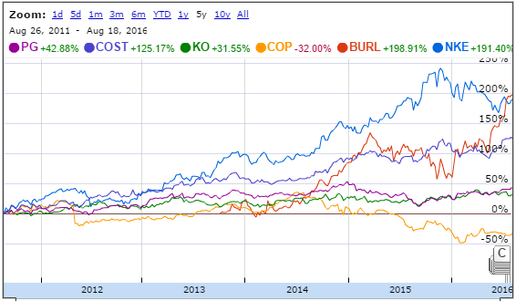
When working with standard investment portfolios, it is necessary to carefully evaluate the current asset status to buy it during the price downward movement.
The first and easiest option for the speculative portfolio trading is a pair trading — creating a spread of two correlating symbols. At Forex, this approach is significantly limited since even highly correlating currency pairs have no cointegration and therefore, can considerably diverge over time. In this case, we deal with a "broken spread". Besides, such pair trading turns into trading a synthetic cross rate since pairs with a common currency are usually included into a spread. This kind of pair trading is a very bad idea. After opening opposite positions by spread, we sometimes have to wait a very long time before the curves converge again.
Below is an example of highly correlating pairs and their gradual and inevitable divergence:
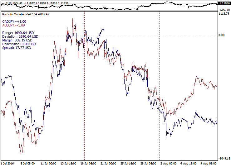
The development of this approach is a multilateral spread trading when three and more currency pairs are included into spread. This is already better than pair trading since it is easier to create a more even spread with greater number of combination options. However, the same risks remain: a spread can diverge and not converge again. It is much easier to achieve good spread return on a quiet market, but strong fundamental news cause a rapid and irreversible divergence after a while. Interestingly, if we increase the number of instruments in a spread, the divergence probability is increased as well, since the more currencies are involved, the greater the probability that something happens during some news release. Waiting for the spread to converge again would be an extremely detrimental strategy, since this works only on a quiet flat market.
Below is a sample multi-lateral spread behavior during a news release:
Spread trading has more opportunities on stock or exchange market in case there is a fundamental connection between assets. However, there are still no guarantees against spread gaps on the dividend date or during futures contracts expiration. Spreads can also be composed of market indices and futures but this requires consideration of exchange trading features.
A dead-end branch of the spread trading is represented by a multi-lock when cyclically related currency pairs (for example, EURUSD-GBPUSD-EURGBP) are selected and used to form a balanced spread. In this case, we have a perfect spread which is impossible to trade since total spreads and commissions are too high. If we try to unbalance lots a bit, the graph becomes more trend-like which contradicts spread trading, while the costs remain high enough making this approach meaningless.
Below is an example of a balanced multi-lock. The total spread is shown as two red lines:
Spread trading drawbacks make us switch to trend models. At first glance, everything seems to be harmonious enough here: identify trend, enter during a correction and exit with profit at higher levels.
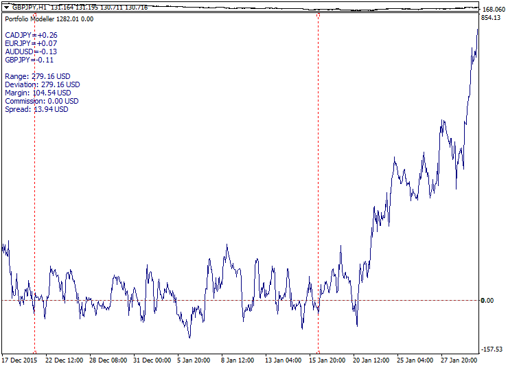
Below is an example of a good trend model:
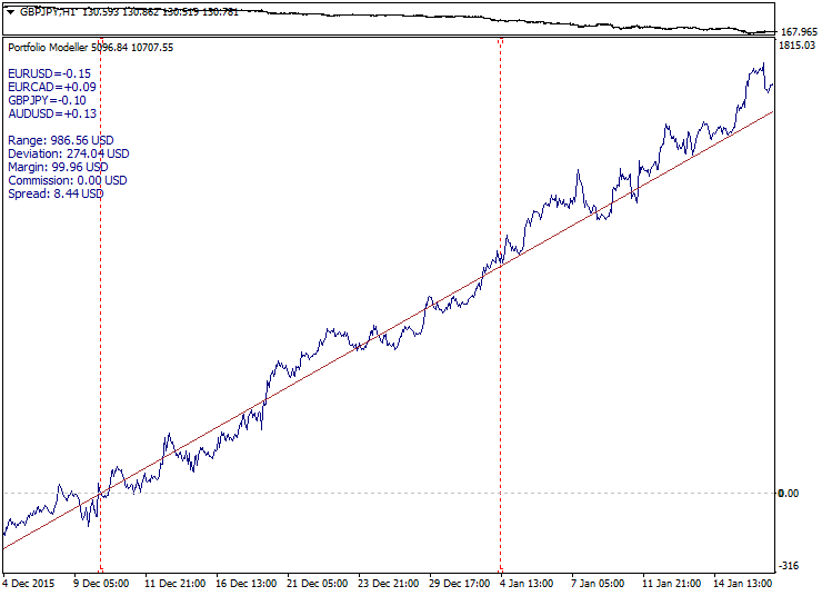
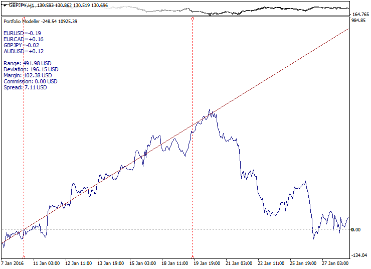
However, trend models may turn out to be not so simple and handy at times. Sometimes, a portfolio refuses to grow further and sometimes it turns down sharply. In this case, we deal with a "broken trend". This occurs quite often on short and medium-term models. The trading efficiency depends heavily on the market phase here. When the market is trendy, the system works well. If the market is flat or especially volatile, numerous losses may occur.
Below you can see a sharp trend completion:
These drawbacks make us reconsider traditional approaches. Now, let's have a look at spread breakout and trend reversal trading methods. The common supposition is that since we cannot avoid portfolio instability, we should learn how to use it.
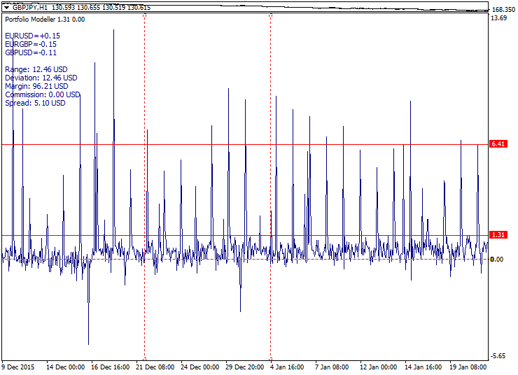
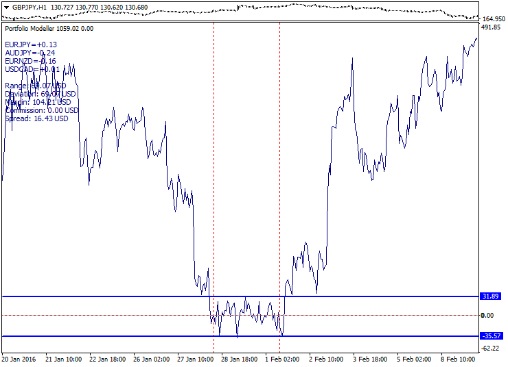
In order to develop a spread breakout setup, we need to create a very compact short-period spread with the minimum volatility in anticipation of a strong movement. The more we compress the portfolio volatility, the stronger it "bursts out". For accelerated spread breakout, it is possible to form a setup before beginning trade sessions and before the news selecting certain intervals of a quiet market. PCA optimization method is best suited for volatility compression. In this setup, we do not know in advance, in which direction the breakout is to occur, therefore, the entry is already defined when moving from the spread boundaries.
Below is a sample exit from the short-period spread channel with the spread channel boundaries highlighted:
The method advantages: short-period spreads are frequent on charts and the volatility after the breakout often exceeds the spread corridor width. The drawbacks: spreads are expanded during news releases and a "saw" may form when the price moves up and down a few times. The conservative entry can be proposed as an alternative after exiting a spread corridor during the correction to the corridor boundary if possible.
In order to create a trend reversal setup, a trend model is created, as well as turning movements and portfolio price levels are tracked. The movement direction is clearly defined but we do not know in advance when the trend reverses. An internal trend line crossing, reverse correction and roll-back are tracked for a conservative entry. Touching an external trend line and a roll-back are tracked for an aggressive entry.
Below is an example of a trend portfolio with the external and internal lines displayed:
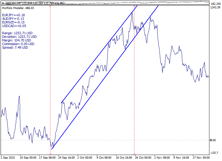
The method advantages: good entry price, convenience, extreme price instability works in favor of the setup. Disadvantages: portfolio price may go up the trend due to fundamental reasons. In order to improve the situation, we may enter in fractional volumes from multiple levels.
A similar setup can be implemented using square root parabolic function model. The setup is based on a well-known property: when the price reaches a theoretical limit of a market distribution range, its further movement is hindered. Like in other cases, the target optimization function is adjusted for the current market distribution. If the markets had featured normal Gaussian distribution, the time-based square root law would have always worked perfectly but since the market distribution is fractal and non-stationary in its nature, the situational adjustment is required.
You can find more about market distributions in the following books by Edgar Peters:
- Chaos and Order in the Capital Markets
- Fractal Market Analysis
Below is an example of a portfolio moving away from the parabolic function:
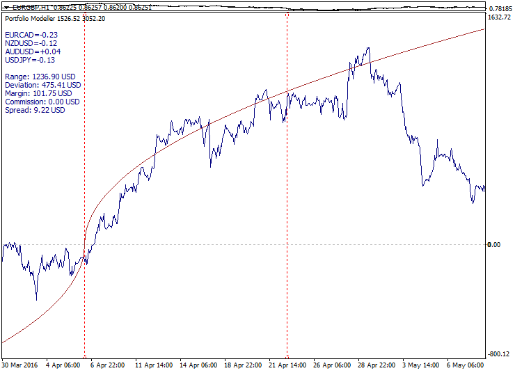
This setup is perfect for adapting to mid-term volatility. However, just like in case of a trend setup, a portfolio price may move upwards due to fundamental factors. The market is not obliged to follow any target function behavior, but neither it is obliged to deviate from it as well. Some degree of freedom and duality remain at all times. All trade setups are not market-neutral in the absolute sense but are based on some form of technical analysis.
The dual nature of trend and flat can be seen below. A trend model looks similar to an uneven flat on a bigger scale:
Apart from symbol combination and model type, location of estimated interval boundaries is of great importance when developing a portfolio. When configuring the portfolio, it might be useful to move the boundaries and compare the results. Good choice of boundaries allows finding portfolios that are more suitable in terms of a trading setup. If a portfolio position enters a drawdown, it is possible to correct the portfolio without closing existing positions. Shifting the boundaries changes the portfolio curve adapting it to a changing situation. Positions should be corrected accordingly after re-arranging the portfolio. This does not mean that the drawdown will decrease in a moment, but the corrected portfolio might become more efficient.
Next, let's consider some properties of portfolio sets and their possible applications in trading systems.
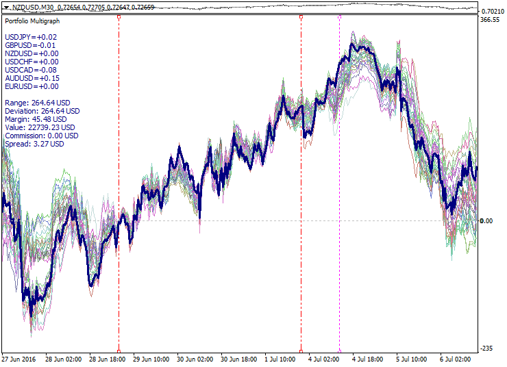
The first property of portfolio sets to catch the eye is a set expansion, or divergence of portfolios with distance from the zero point. It would be only natural and reasonable to use this property for trading: buying rising portfolios and selling falling ones.
Below is a sample expanding set of portfolios:
The second property — portfolio set compression (convergence) — is opposite to the previous one. It happens after an expansion. Expansion and compression cycles suggest that this behavior can be used to open synthetic positions in anticipation of returning to the center of the set after reaching an alleged highest degree of expansion. However, the expansion highest degree always vary, and it is impossible to predict the final boundaries of the set curves expansion.
Below is a sample compressing set of portfolios:
Applying various target functions, filtration parameters, reversals and combinations provides good opportunities for experimenting and searching for efficient trading setups. Generally, all setups can be divided into two classes: trading breakouts and trading roll-backs.
Below is an example of the first type trading setup with a reversal and shift of a portfolio set:

A sample roll-back trading setup based on the multi-trend model is provided below:
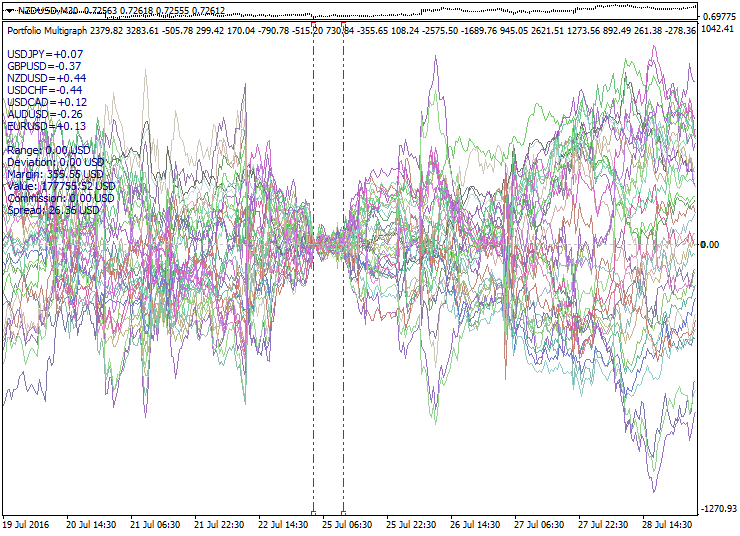
Another recurring portfolio property is a set twist (self-crossing). Typically, this corresponds to a change of a market trend. If we trade in anticipation of an expansion of portfolios, a twist is a negative effect requiring the set re-arrangement. For other strategies, crossing of some portfolio curves can be used to identify promising and played-out portfolios. Besides, it is necessary to consider a distance traveled, levels, position in a set and position relative to the target function.
Below is an example of a set twisting multiple times:
We have not focused out attention on the volume management issue up until now, though this is a critical part of any trading system. Generally, we can describe the following approaches:
- trading a single synthetic position (the simplest case)
- dividing the volumes (extended entry by levels)
- adding to a rising portfolio (pyramiding by trend)
- adding to a portfolio in a drawdown (position averaging)
- adding to a portfolio after a correction (finishing method)
- adding to a portfolio after a reversal (expansive strategy)
- adding to new portfolios (portfolio consolidation)
- combined approach (combining several approaches)
Specific volume management method should be selected considering trading system features. When planning a profit and a drawdown, your calculations should be based on a portfolio volatility. In the simplest case, the portfolio volatility can be evaluated as the movement range of its graph within a certain segment. It is much better to evaluate volatility not only within the optimization interval but on the previous history as well. Knowing the portfolio volatility, it is possible to calculate a theoretical value of the maximum total drawdown at a series of positions. Traditionally, we caution against too frequent aggressive volume adding. The total funds allocated for a portfolio coverage on a trading account should be able to withstand unfavorable movement considering all additional positions.
Multi-portfolio trading means systematic portfolio selection and consolidation. If one portfolio is bought and another one is added to it, this may have a positive diversification effect if the portfolios have noticeable differences. But if portfolios are correlating, this may have a negative effect, since they both may find themselves in a drawdown in case of an unfavorable movement. Normally, you should avoid adding correlating portfolios. At first glance, trading spread between two correlating portfolios may seem to be very promising but closer examination shows that such spreads are no different from usual spreads since they are not stationary.
Various exit strategies can be applied in multi-portfolio trading, including:
- closing by total result of all portfolios
- closing a group of portfolios by the group's total result
- closing by certain portfolios' targets and limits.
For some strategies, the entry point is of critical importance. For example, if a strategy applies extreme prices before a trend reversal or correction, a period suitable for entry is very short. Other strategies are more reliant on the optimal calculation of a position adding system and portfolio selection principle. In this case, individual portfolios may enter a drawdown, but other (more efficient) portfolios within the consolidated series adjust the overall result.
Conclusion
Portfolio trading advantages: optimization allows you to create a portfolio curve according to your preferences, as well as form a desired trading setup and trade it similar to trading symbols on a price chart. However, unlike trading portfolios, buying and selling conventional assets leave traders in passive position (since they are only able to accept the current price chart or avoid using it). Besides, as the situation evolves, traders can adjust their portfolios to new market conditions.
Portfolio trading drawbacks: standard pending orders are not applicable, more stringent minimum volume requirements, bigger spreads on М30 and lower charts, hindered intraday scalping, no OHLC data, not all indicators can be applied to portfolios.
Generally, this is a rather specific approach in trading. Here we have only made an introductory overview of the portfolio properties and working methods. If you want to perform deeper studies of portfolio trading systems, I recommend using the MetaTrader 5 platform for that, while market distribution properties should be studied in specialized statistical packages.
Translated from Russian by MetaQuotes Ltd.
Original article: https://www.mql5.com/ru/articles/2646
Warning: All rights to these materials are reserved by MetaQuotes Ltd. Copying or reprinting of these materials in whole or in part is prohibited.
This article was written by a user of the site and reflects their personal views. MetaQuotes Ltd is not responsible for the accuracy of the information presented, nor for any consequences resulting from the use of the solutions, strategies or recommendations described.

 The Easy Way to Evaluate a Signal: Trading Activity, Drawdown/Load and MFE/MAE Distribution Charts
 LifeHack for trader: "Quiet" optimization or Plotting trade distributions
 Working with currency baskets in the Forex market
 MQL5 vs QLUA - Why trading operations in MQL5 are up to 28 times faster?
- Free trading apps
- Over 8,000 signals for copying
- Economic news for exploring financial markets
You agree to website policy and terms of use
This article is just mind boggling! And this is just an introduction?? Wow!
Why?
In both cases, I'd recommend not to skip the References of 1. and the References of 2.
For getting a better idea of the challenges to be mastered one may have a look at the video on a Full Time Trader's preferred trading style even though I point out my
After all, it is not by chance that professionals usually aim for Delta neutral portfolios.
The only recommendation I actually can give is to understand as much of the page Risk-Neutral Measure as possible!
This is very interesting article, thank you.
Personaly I like more working with external software for creating and evaluating portfolio with correlation and other statistics more, than adjusting or programming Metatrader. But idea stays the same, do not use single strategy, but rather portfolio of matching strategies for better sustainability.