
The Role of Statistical Distributions in Trader's Work
Regularities make our life easier but it's as important to benefit from randomness.
(Georgiy Aleksandrov)
Introduction
This article is a logical continuation of my article Statistical Probability Distributions in MQL5 which set forth the classes for working with some theoretical statistical distributions. I found it necessary to first lay the foundation in the form of distribution classes in order to make it more convenient for a user to utilize them afterwards in practice.
Now that we have a theoretical base, I suggest that we should directly proceed to real data sets and try to make some informational use of this base. At the same time we will throw light upon some issues relating to mathematical statistics.
1. Generation Of Random Numbers With A Given Distribution
But before considering real data sets, it appears very important to be able to get some set of values that would be closely related to a desired theoretical distribution.
In other words, a user should only set parameters of the desired distribution and sample size. A program (in our case, a hierarchy of classes) should generate and output such sample of values for further work.
Another significant detail is that samples generated by a specified law are used to check various statistical tests. The area of mathematical statistics - generation of random variables with different distribution laws - is quite interesting and challenging.
For my purposes, I used a high quality generator described in the book Numerical Recipes: The Art of Scientific Computing [2]. Its period approximately equals to 3.138*1057. C code was quite easily passed into MQL5.
And so I created the Random class, as follows:
//+------------------------------------------------------------------+
//|                    Random class definition                       |
//+------------------------------------------------------------------+
class Random
  {
private:
   ulong u, //unsigned 64-bit integers
   v,
   w;
public:
   //+------------------------------------------------------------------+
   //| The Random class constructor                                      |
   //+------------------------------------------------------------------+
   void Random()
     {
      randomSet(184467440737095516);
     }
   //+------------------------------------------------------------------+
   //| The Random class set-method                                      |
   //+------------------------------------------------------------------+
   void randomSet(ulong j)
     {
      v=4101842887655102017;
      w=1;
      u=14757395258967641292;
      u=j^v;
      int64();
      v = u; int64();
      w = v; int64();
     }
   //+------------------------------------------------------------------+
   //| Return 64-bit random integer                                     |
   //+------------------------------------------------------------------+
   ulong int64()
     {
      uint k=4294957665;
      u=u*2862933555777941757+7046029254386353087;
      v^= v>> 17; v ^= v<< 31; v ^= v>> 8;
      w = k*(w & 0xffffffff) +(w>> 32);
      ulong x=u^(u<<21); x^=x>>35; x^=x<<4;
      return(x+v)^w;
     };
   //+------------------------------------------------------------------+
   //| Return random double-precision value in the range 0. to 1.       |
   //+------------------------------------------------------------------+
   double doub()
     {
      return 5.42101086242752217e-20*int64();
     }
   //+------------------------------------------------------------------+
   //| Return 32-bit random integer                                     |
   //+------------------------------------------------------------------+
   uint int32()
     {
      return(uint)int64();
     }
  };
We can now create classes for values sampled from a distribution.
As an example, let us have a look at a random variable from the normal distribution. The CNormaldev class is, as follows:
//+------------------------------------------------------------------+
//|                    CNormaldev class definition                   |
//+------------------------------------------------------------------+
class CNormaldev : public Random
  {
public:
   CNormaldist       N; //Normal Distribution instance
   //+------------------------------------------------------------------+
   //| The CNormaldev class constructor                                 |
   //+------------------------------------------------------------------+
   void CNormaldev()
     {
      CNormaldist Nn;
      setNormaldev(Nn,18446744073709);
     }
   //+------------------------------------------------------------------+
   //| The CNormaldev class set-method                                  |
   //+------------------------------------------------------------------+
   void setNormaldev(CNormaldist &Nn,ulong j)
     {
      N.mu=Nn.mu;
      N.sig=Nn.sig;
      randomSet(j);
     }
   //+------------------------------------------------------------------+
   //| Return  Normal deviate                                           |
   //+------------------------------------------------------------------+
   double dev()
     {
      double u,v,x,y,q;
      do
        {
         u = doub();
         v = 1.7156*(doub()-0.5);
         x = u - 0.449871;
         y = fabs(v) + 0.386595;
         q = pow(x,2) + y*(0.19600*y-0.25472*x);
        }
      while(q>0.27597
      && (q>0.27846 || pow(v,2)>-4.*log(u)*pow(u,2)));
      return N.mu+N.sig*v/u;
     }
  };
//+------------------------------------------------------------------+
As can be seen, the class has a data member N of CNormaldist type. The original C code lacked such connection with the distribution. I considered it necessary for a random variable generated by the class (here, by CNormaldev class) to have a logical and programmatic connection with its distribution.
In the original version, Normaldev type was defined, as follows:
typedef double Doub;
typedef unsigned __int64 Ullong;

struct Normaldev : Ran
{
 Doub mu,sig;
 Normaldev(Doub mmu, Doub ssig, Ullong i)
...
}
Random numbers are generated here from the normal distribution using Leva's ratio of uniforms method.
All other classes that assist in calculation of random variables from various distributions, are situated in the include Random_class.mqh file.
We will now finish with generation and see, in practical part of the article, how to create an array of values and test a sample.
2. Estimation Of Distribution Parameters, Statistical Hypotheses
It is clear that we will look into discrete variables. In practice however, if the number of discrete variables is significant, it is more convenient to consider the set of such discrete variables as a group of continuous variables. This is a standard approach in mathematical statistics. Therefore for their analysis we can use distributions defined by analytical formulas that are related to continuous variables.
So let us get down to the analysis of the empirical distribution.
It is assumed that a sample of a general population whose members meet the criterion of representativeness is under study. In addition, the requirements to the estimates specified in Section 8.3 [9] are met. Numeric distribution parameters can be found by means of point estimation and interval methods.
2.1 Sample Handling Using The CExpStatistics Class
One should first delete the so-called outliers from the sample; these are observations that deviate markedly from observations of the major part of the sample (both upward and downward). There is no universal method for deleting the outliers.
I suggest using the one described by S.V. Bulashev in Section 6.3 [5]. In MQL4 forum, a library of statistical functions was created on the basis of which the given problem can easily be solved. That said, we will surely apply OOP and update it a little bit.
I called the created class of estimates of statistical characteristics CExpStatistics (Class of Expected Statistics).
It roughly is, as follows:
//+------------------------------------------------------------------+
//|             Expected Statistics class definition                 |
//+------------------------------------------------------------------+
class CExpStatistics
  {
private:
   double            arr[];      //initial array
   int               N;          //initial array size
   double            Parr[];     //processed array
   int               pN;         //processed array size
   void              stdz(double &outArr_st[],bool A); //standardization
public:
   void              setArrays(bool A,double &Arr[],int &n); //set array for processing
   bool              isProcessed;  //array processed?
   void              CExpStatistics(){};  //constructor
   void              setCExpStatistics(double &Arr[]); //set the initial array for the class
   void              ZeroCheckArray(bool A); //check the input array for zero elements
   int               get_arr_N();           //get the initial array length
   double            median(bool A);         //median
   double            median50(bool A); //median of 50% interquantile range (midquartile range)
   double            mean(bool A);     //mean of the entire initial sample
   double            mean50(bool A);   //mean of 50% interquantile range
   double            interqtlRange(bool A); //interquartile range
   double            RangeCenter(bool A); //range center
   double            meanCenter(bool A);  //mean of the top five estimates
   double            expVariance(bool A); //estimated variance
   double            expSampleVariance(bool A); //shifted estimate of sample variance
   double            expStddev(bool A);   //estimated standard deviation
   double            Moment(int index,bool A,int sw,double xm); //moment of distribution
   double            expKurtosis(bool A,double &Skewness); ////estimated kurtosis and skewness
   double            censorR(bool A); //censoring coefficient
   int               outlierDelete(); //deletion of outliers from the sample
   int               pArrOutput(double &outArr[],bool St); //processed array output
   void              ~CExpStatistics(){};//destructor
  };
//+------------------------------------------------------------------+
Implementation of each method can be studied in detail in the include ExpStatistics_class.mqh file so I will leave it out here.
The important thing this class does is that it returns the array free of outliers (Parr[]), if any. Besides, it helps in getting some descriptive statistics of sampling and their estimates.
2.2 Creating A Processed Sample Histogram
Now that the array is free of outliers, a histogram (frequency distribution) can be drawn based on its data. It will help us to visually estimate the random variable distribution law. There is a step-by-step procedure for creating a histogram.
One should first calculate the number of required classes. In this context, the term "class" means grouping, interval. The number of classes is calculated by Sturges' formula:

Where k is the number of classes, n is the number of observations.
In MQL5 the formula may be represented, as follows:
int Sturges(int n)
/*
   Function for determining the number of class intervals using Sturges' rule.
   Variables:
     y is the number of sampling observations.
   Returned value:
     number of class intervals.
*/
{
   double s;        // Returned value
   s=1.+log2(y);
   if(s>15)         // Empirical rule
      s=15;
   return(int) floor(s);
}
When the required number of classes (intervals) has been received using Sturges' formula, it is time to break down the array data into classes. Such data is called observations (sing. observation). We will do it using the Allocate function, as follows:
void  Allocate(double &data[],int n,double &f[],double &b[],int k)
/*
  Function for allocating observations to classes.
  Variables:
   1) data — initial sample (array)
   2) n — sample size
   3) f — calculated array of observations allocated to classes
   4) b — array of class midpoints
   5) k — number of classes
*/
  {
   int i,j;                     // Loop counter
   double t,c;                  // Auxiliary variable
   t=data[ArrayMinimum(data)]; // Sample minimum
   t=t>0 ? t*0.99 : t*1.01;
   c=data[ArrayMaximum(data)]; // Sample maximum
   c=c>0 ? c*1.01 : c*0.99;
   c=(c-t)/k/2;                // Half of the class interval
   b[0]=t+c;                   // Array of class interval midpoints
   f[0]= 0;
   for(i=1; i<k; i++)
     {
      b[i] = b[i - 1] + c + c;
      f[i] = 0;
     }
// Grouping
   for(i=0; i<n; i++)
      for(j=0; j<k; j++)
         if(data[i]>b[j]-c && data[i]<=b[j]+c)
           {
            f[j]++;
            break;
           }
  }
As can be seen, the function takes in the array of initial observations (data), its length (n), number of classes (k) and allocates the observations to a certain f[i] class of the f array, where b[i] is the f[i] class midpoint. The histogram data is now ready.
We will display the histogram using the tools described in the previously mentioned article. For this purpose I wrote the histogramSave function which will display the histogram for the series under study in HTML. The function takes in 2 parameters: array of classes (f) and array of class midpoints (b).
As an example, I built a histogram for absolute differences between maximums and minimums of 500 bars of the EURUSD pair on the four-hour time frame in points using the volatilityTest.mq5 script.
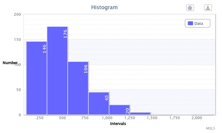
Figure 1. Data histogram (absolute volatility of the EURUSD H4)
As shown in the histogram (Fig. 1), the first class has 146 observations, the second class has 176 observations, etc. The function of the histogram is to give a visual idea of the empirical distribution of the sample under study.
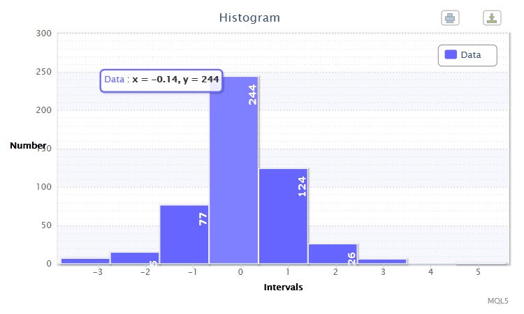
Figure 2. Data histogram (standardized returns of the EURUSD H4)
The other histogram (Fig.2) displays standardized logarithmic returns of 500 bars of the EURUSD pair on the H4 timeframe. As you can notice, the fourth and fifth classes are the most impressive as they have got 244 and 124 observations, respectively. This histogram was built using the returnsTest.mq5 script.
So, the histogram enables us to choose the distribution law the parameters of which will be further estimated. Where it is not visually obvious which distribution to prefer, you can estimate parameters of several theoretical distributions.
Both distributions we considered do not resemble the normal ones in appearance, especially the first one. However let us not trust the visual representation and proceed to figures.
2.3 Hypothesis Of Normality
It is customary to first solve and test the assumption (hypothesis) of whether the distribution in question is normal. Such hypothesis is called the main hypothesis. One of the most popular methods for testing the normality of a sample is the Jarque-Bera test.
Its algorithm, although not most complex, is quite bulky due to approximation. There is a few versions of the algorithm in C++ and other languages. One of the most successful and proven versions is a version situated in a cross-platform numerical analysis library ALGLIB. Its author [S.A. Bochkanov] did a huge job, particularly in compilation of the test quantile table. I just updated it slightly to the needs of MQL5.
The main function jarqueberatest is, as follows:
//+------------------------------------------------------------------+
//                   the Jarque-Bera Test                            |
//+------------------------------------------------------------------+
void jarqueberatest(double &x[],double &p)
/*
  The Jarque-Bera test is used to check hypothesis about the fact that
   a given sample xS  is a sample of normal random variable with unknown
   mean and variance.
   Variables:
     x - sample Xs;
     p - p-value;
*/
  {
   int n=ArraySize(x);
   double s;
   p=0.;
   if(n<5)//N is too small
     {
      p=1.0;
      return;
     }
//N is large enough
   jarquebera_jarqueberastatistic(x,n,s);
   p=jarquebera_jarqueberaapprox(n,s);
  }
//+------------------------------------------------------------------+
It treats the initial data sample (x) and returns the р-value, i.e. a value that characterizes the probability of rejecting a null hypothesis if the null hypothesis is in fact true.
There are 2 auxiliary functions in the function body. The first function - jarquebera_jarqueberastatistic - calculates the Jarque-Bera statistic, and the second one - jarquebera_jarqueberaapprox - calculates the p-value. It should be noted that the latter, in its turn, brings into action auxiliary functions related to approximation, which are almost 30 in the algorithm.
So let us try to test our samples for normality. We will use the returnsTest.mq5 script that will treat the sample of standardized returns of the EURUSD H4.
As expected, the test showed that the probability of rejecting a true null hypothesis is 0.0000. In other words, the distribution of this sample does not belong to the family of normal distributions. In order to treat the sample of absolute volatility of the EURUSD pair, run the volatilityTest.mq5 script. The result will be similar - the distribution is not normal.
3. Distribution Fitting
There is a few methods in mathematical statistics that allow for comparing the empirical distribution with the normal distribution. The biggest problem is that the normal distribution parameters are not known to us and there is an assumption that the data under study does not reflect the normality of a distribution.
Therefore we have to use nonparametric tests and fill the unknown parameters with the estimates obtained from the empirical distribution.
3.1 Estimation And Testing
One of the most popular and, what's most important, adequate tests in this situation is χ2 test. It is based on Pearson's goodness of fit measure.
We will perform the test using the chsone function:
void chsone(double &f[],double &ebins[],double &df,
            double &chsq,double &prob,const int knstrn=1)
/*
   1) f — array of observations allocated to classes
   2) ebins - array of expected frequencies
   3) df - number of degrees of freedom
   3) chsq — chi-square statistics
   4) prob - probability of accepting a true null hypothesis
   5) knstrn — constraint
*/
  {
   CGamma gam;
   int j,nbins=ArraySize(bins),q,g;
   double temp;
   df=nbins-knstrn;
   chsq=0.0;
   q=nbins/2;
   g=nbins-1;
   for(j=0;j<nbins/2;j++) //passing through the left side of the distribution
     {
      if(ebins[j]<0.0 || (ebins[j]==0. && bins[j]>0.))
         Alert("Bad expected number in chsone!");
      if(ebins[j]<=5.0)
        {
         --df;
         ebins[j+1]+=ebins[j];
         bins[j+1]+=bins[j];
        }
      else
        {
         temp=bins[j]-ebins[j];
         chsq+=pow(temp,2)/ebins[j];
        }
     }
   for(j=nbins-1;j>nbins/2-1;j--) //passing through the right side of the distribution
    {
      if(ebins[j]<0.0 || (ebins[j]==0. && bins[j]>0.))
         Alert("Bad expected number in chsone!");
      if(ebins[j]<=5.0)
        {
         --df;
         ebins[j-1]+=ebins[j];   //starting with the last class
         bins[j-1]+=bins[j];
        }
      else
        {
         temp=bins[j]-ebins[j];
         chsq+=pow(temp,2)/ebins[j];
        }
     }
   if(df<1)df=1; //compensate
   prob=gam.gammq(0.5*df,0.5*chsq); //Chi-square probability function
  }
As can be seen in the listing, an instance of the CGamma class is used representing the incomplete gamma function which is included in the Distribution_class.mqh file as well as all the mentioned distributions. It should also be noted that the array of expected frequencies (ebins) will be obtained by using the estimateDistribution and expFrequency functions.
We now need to select the numerical parameters that are included in the analytical formula for the theoretical distribution. The number of parameters depends on the particular distribution. For example, there are two parameters in the normal distribution, and one parameter in the exponential distribution, etc.
When determining the distribution parameters we usually use such point estimation methods as the method of moments, quantile method and maximum likelihood method. The first one is simpler as it implies that the sampling estimates (expectation, variance, skewness, etc.) should coincide with the general estimates.
Let us try to select a theoretical distribution for our sample using an example. We are going to take a series of standardized returns of the EURUSD H4 for which we have already drawn a histogram.
First impression is that the normal distribution is not appropriate for the series as the excess coefficient of kurtosis is observed. As a comparison, let us try to apply another distribution.
So, when starting the already known returnsTest.mq5 script, we are going to try selecting such distribution as Hypersec. In addition, the script will estimate and output the selected distribution parameters using the estimateDistribution function and immediately run the χ2 test. The selected distribution parameters have turned out to be, as follows:
Hyperbolic Secant distribution: X~HS(-0.00, 1.00);
and the test results were, as follows:
"Chi-square statistic: 1.89; probability of rejecting a true null hypothesis: 0.8648"
It should be noted that the selected distribution is a good fit as the value of the χ2 statistic is quite small.
Moreover, using the histogramSaveE function a double histogram for the observed and expected frequency ratios (frequency ratio is a frequency expressed in fraction or percent) of standardized returns will be drawn (Fig. 3). You can see that the bars nearly duplicate each other. This is a proof of the successful fitting.
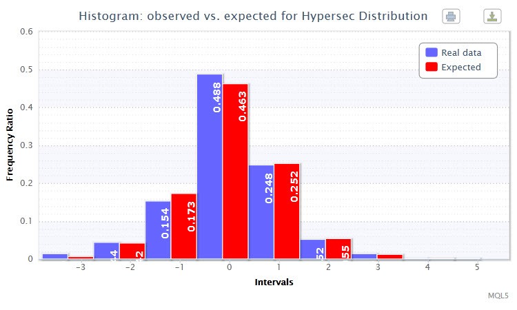
Figure 3. Histogram of the observed and expected frequency ratios (standardized returns of the EURUSD H4)
Let us carry out a similar procedure for volatility data using the already known volatilityTest.mq5.
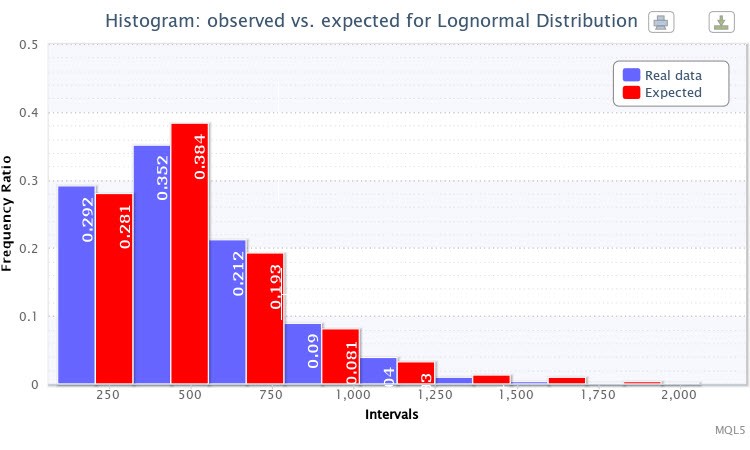
Figure 4. Histogram of the observed and expected frequency ratios (absolute volatility of the EURUSD H4)
I selected the lognormal distribution Lognormal for testing. As a result, the following estimation of the parameters was received:
Lognormal distribution: X~Logn(6.09, 0.53);
and the test results were, as follows:
"Chi-square statistic: 6.17; probability of rejecting a true null hypothesis: 0.4040"
The theoretical distribution for this empirical distribution was also quite successfully selected. Thus, one can consider that the null hypothesis cannot be rejected (at the standard confidence level p=0.05). One can see in Fig. 4 that the bars of the expected and observed frequency ratios are also very much alike.
Let me now remind you that we have another possibility to generate a sample of random variables from a distribution with set parameters. In order to use a hierarchy of classes related to such operation, I wrote the randomTest.mq5 script.
At the start thereof, we need to enter the parameters as shown in Fig. 5.
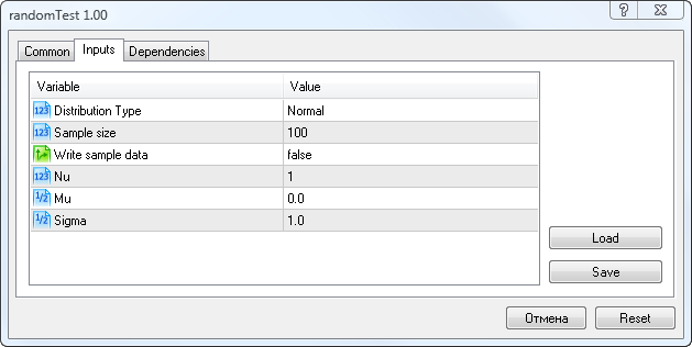
Figure 5. Input parameters of the randomTest.mq5 script
Here you can select the distribution type (Distribution Type), the number of random variables in a sample (Sample Size), the sample saving option (Write sample data), the Nu parameter (for the Student's t-distribution), the Mu and Sigma parameters.
If you set for Write sample data the value true, the script will save the sample of random variables with the custom parameters to the Randoms.csv file. Otherwise it will read the sample data from this file and then perform statistical tests.
For some distributions with missing Mu and Sigma parameters, I've provided a table of parameter correlation to the fields in the script start window.
| Distribution | First distribution parameter | Second distribution parameter |
|---|---|---|
| Logistic | alph --> Mu | bet --> Sigma |
| Exponential | lambda --> Mu | -- |
| Gamma | alph --> Mu | bet --> Sigma |
| Beta | alph --> Mu | bet --> Sigma |
| Laplace | alph --> Mu | bet --> Sigma |
| Binomial | n --> Mu | pe --> Sigma |
| Poisson | lambda --> Mu | -- |
For instance, if the Poisson distribution is selected, the lambda parameter will be entered through Mu field, etc.
The script does not estimate the Student's t-distribution parameters because in the absolute majority of cases it is only used in a few statistical procedures: point estimation, building of confidence intervals and testing of hypotheses that concern the unknown mean of a statistical sample from the normal distribution.
As an example, I ran the script for the normal distribution with the parameters X~Nor(3.50, 2.77) where Write sample data=true. The script first generated a sample. Upon the second run at Write sample data=false, a histogram was drawn as shown in Fig.6.
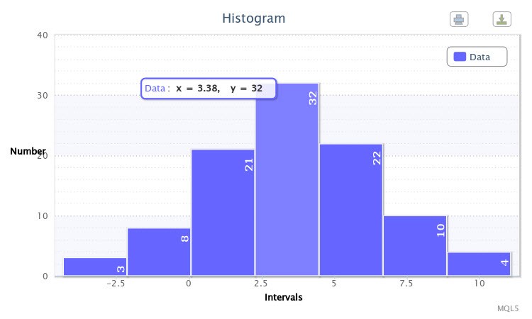
Figure 6. The sample of random variables X~Nor(3.50,2.77)
The remaining information displayed in the Terminal window is, as follows:
The Jarque-Bera test: "The Jarque-Bera test: probability of rejecting a true null hypothesis is 0.9381";
Parameter estimation: Normal distribution: X~Nor(3.58, 2.94);
Chi-square test results: "Chi-square statistic: 0.38; probability of rejecting a true null hypothesis: 0.9843".
And finally, another double histogram of the observed and expected frequency ratios for the sample was displayed (Fig. 7).
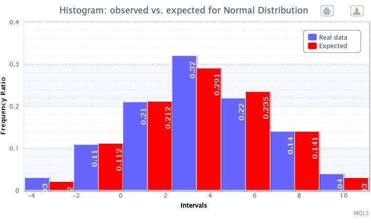
Figure 7. Histogram of the observed and expected frequency ratios for X~Nor(3.50,2.77)
In general, the generation of the specified distribution was successful.
I also wrote the fitAll.mq5 script that works in a way similar to the randomTest.mq5 script. The only difference is that the first one has the fitDistributions function. I set the following task: to fit all available distributions to a sample of random variables and perform a statistical test.
It is not always possible to fit a distribution to a sample due to the parameter mismatch that leads to the appearance of lines in the Terminal informing that the estimation is not possible, e.g. "Beta distribution cannot be estimated!".
Further, I decided that this script should visualize statistical results in the form of a small HTML report an example of which can be found in article "Charts and Diagrams in HTML" (Fig. 8).
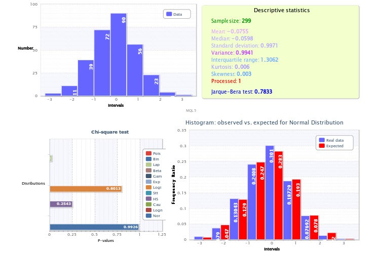
Figure 8. Statistical report on sample estimation
A standard histogram of the sample is displayed in the top left quarter; the top right quarter represents the descriptive statistics and Jarque-Bera test result, where the Processed variable value equal to 1 means that the outliers were deleted while a value of 0 means that there were no outliers.
P-values of the χ2 test for every selected distribution are displayed in the bottom left quarter. Here, the normal distribution turned out to be the best in terms of fitting (p=0.9926). Therefore a histogram of the observed and expected frequency ratios was drawn for it in the bottom right quarter.
There are not so many distributions in my gallery as yet. But this script will save you a lot of time if there is a great number of distributions.
Now that we know exactly the distribution parameters of samples under study, we can proceed to probabilistic reasoning.
3.2 Probabilities Of Random Variable Values
In the article about theoretical distributions I gave the continuousDistribution.mq5 script as an example. Using it, we will try to display any distribution law with known parameters which can be of interest to us.
So, for volatility data we will enter the lognormal distribution parameters obtained earlier (Mu=6.09, Sigma=0.53), select the Lognormal distribution type and cdf mode (Fig.9).
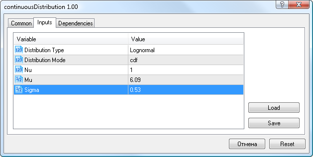
Figure 9. Lognormal distribution parameters X~Logn(6.09,0.53)
The script will then display the distribution function for our sample. It will appear as shown in Fig. 10.
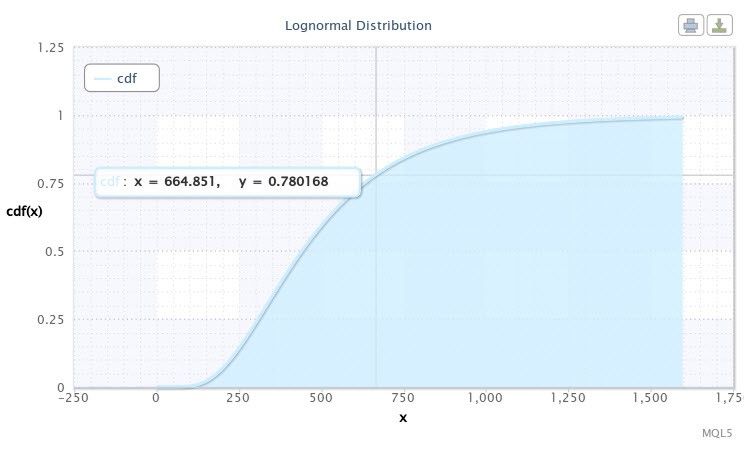
Figure 10. Distribution function for X~Logn(6.09,0.53)
We can see in the chart that the cursor is pointed at a point the coordinates of which approximately are [665;0.78]. It means that there is a 78% probability that volatility of the EURUSD H4 will not exceed 665 points. This information may prove to be very useful for a developer of an Expert Advisor. One can surely take other values on the curve by moving the cursor.
Let us assume that we are interested in probability of the event when the volatility value will lie in the interval between 500 and 750 points. For this purpose the following operation needs to be performed:
cdf(750) - cdf(500) = 0.84 - 0.59 = 0.25.
Thus, in a fourth of events the volatility of the pair fluctuates in the interval between 500 and 750 points.
Let us run the script with the same distribution parameters once again only selecting sf as a mode of distribution law. The reliability (survival) function will be shown, as follows (Fig.11).
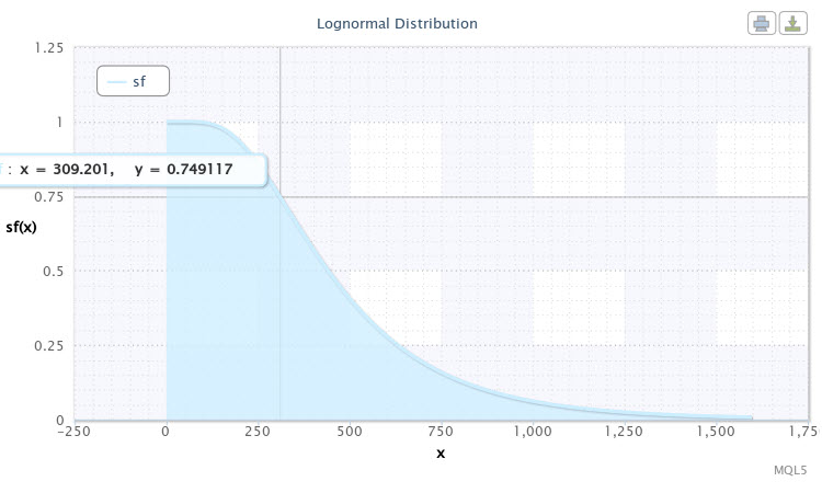
Figure 11. The survival function for X~Logn(6.09,0.53)
The point marked in the curve chart can be interpreted, as follows: we can expect with nearly 75% probability that volatility of the pair will be 310 points. The lower we go down the curve, the lesser the probability of volatility to increase. Thus, volatility of over 1000 points may already be considered a rare event as the probability of the occurrence thereof is less than 5%.
Similar distribution curves can be built for the sample of standardized returns as well as for other samples. I suppose the methodology is generally clear.
Conclusion
It should be noted that the proposed analytical derivations are not entirely successful as series tend to vary. Although, for instance, it does not concern series of logarithmic returns. However I didn't set myself a task of evaluating the methods in this article. I suggest that the interested reader comment on this issue.
It is important to note the need to consider the market, market instruments and trade experts from probability perspective. This is the approach I have tried to demonstrate. I hope this subject will arouse the reader's interest and lead to a constructive discussion.
Location of files:
| # | File | Path | Description |
|---|---|---|---|
| 1 | Distribution_class.mqh | %MetaTrader%\MQL5\Include | Gallery of distribution classes |
| 2 | DistributionFigure_class.mqh | %MetaTrader%\MQL5\Include | Classes for graphical display of distributions |
| 3 | Random_class.mqh | %MetaTrader%\MQL5\Include | Classes for generation of a random number sample |
| 4 | ExpStatistics_class.mqh | %MetaTrader%\MQL5\Include | Class and functions of estimates of statistical characteristics |
| 5 | volatilityTest.mq5 | %MetaTrader%\MQL5\Scripts | Script for estimation of the EURUSD H4 volatility sample |
| 6 | returnsTest.mq5 | %MetaTrader%\MQL5\Scripts | Script for estimation of the EURUSD H4 returns sample |
| 7 | randomTest.mq5 | %MetaTrader%\MQL5\Scripts | Script for estimation of the random variable sample |
| 8 | fitAll.mq5 | %MetaTrader%\MQL5\Scripts | Script for fitting and estimation of all distributions |
| 9 | Volat.csv | %MetaTrader%\MQL5\Files | EURUSD H4 volatility sample data file |
| 10 | Returns_std.csv | %MetaTrader%\MQL5\Files | EURUSD H4 returns sample data file |
| 11 | Randoms.csv | %MetaTrader%\MQL5\Files | Random variable sample data file |
| 12 | Histogram.htm | %MetaTrader%\MQL5\Files | Histogram of the sample in HTML |
| 13 | Histogram2.htm | %MetaTrader%\MQL5\Files | Double histogram of the sample in HTML |
| 14 | chi_test.htm | %MetaTrader%\MQL5\Files | Statistical HTML report of the sample estimation |
| 15 | dataHist.txt | %MetaTrader%\MQL5\Files | Data for displaying a histogram of samples |
| 16 | dataHist2.txt | %MetaTrader%\MQL5\Files | Data for displaying a double histogram of samples |
| 17 | dataFitAll.txt | %MetaTrader%\MQL5\Files | Data for HTML report display |
| 18 | highcharts.js | %MetaTrader%\MQL5\Files | JavaScript library of interactive charts |
| 19 | jquery.min.js | %MetaTrader%\MQL5\Files | JavaScript library |
| 20 | ReturnsIndicator.mq5 | %MetaTrader%\MQL5\Indicators | Logarithmic returns indicator |
Reference Materials:
Translated from Russian by MetaQuotes Ltd.
Original article: https://www.mql5.com/ru/articles/257
Warning: All rights to these materials are reserved by MetaQuotes Ltd. Copying or reprinting of these materials in whole or in part is prohibited.
This article was written by a user of the site and reflects their personal views. MetaQuotes Ltd is not responsible for the accuracy of the information presented, nor for any consequences resulting from the use of the solutions, strategies or recommendations described.
 Universal Regression Model for Market Price Prediction
 Custom Graphical Controls. Part 3. Forms
 Creating Expert Advisors Using Expert Advisor Visual Wizard
 Object-Oriented Approach to Building Multi-Timeframe and Multi-Currency Panels
- Free trading apps
- Over 8,000 signals for copying
- Economic news for exploring financial markets
You agree to website policy and terms of use
I like your opinion about the applicability of scientific knowledge in trading.
Could you please tell me which of the books you would recommend to a person who is familiar with probability theory and mathematical statistics?
Denis, good afternoon.
I like your opinion about the applicability of scientific knowledge in trading.
Please tell me which of the books you would recommend to a person who is familiar with probability theory and mathematical statistics.
Thank you for your opinion!
I think that one should look for something for beginners then, some lit-role. The main thing is that the text of the book should not discourage you from reading it further :-))).
I liked something Gaidyshev, and something Bulashev.....
There's an interesting threadhere.
The second inaccuracy is that you have not used the a priori knowledge that the top (aka expectation) of the distribution of returns must be exactly at 0 (otherwise we would all have been billionaires long ago).
Not at all. A shift of the top of the distribution relative to 0 (growth/decline of an instrument) does not mean that it will be the same in the future. That is why most traders are not billionaires, not because.
Regards.
...Shifting the top of the distribution relative to 0 (rising/falling instrument) does not necessarily mean that this will be the case in the future...
Agreed.
Question for alsu. Did you mean market efficiency when talking about the zero point?
Dear Mr. Dennis Kirichenko
I get some warning when I compile file continuousDistribution.mq5 "declaration of 'nn' hides global declaration in file 'continuousDistribution.mq5' at line 27 DistributionFigure_class.mqh 107 57".
"declaration of 'mm' hides global declaration in file 'continuousDistribution.mq5' at line 27 DistributionFigure_class.mqh 107 57"
"declaration of 'ss' hides global declaration in file 'continuousDistribution.mq5' at line 27 DistributionFigure_class.mqh 107 57"
Can you fix it ??? Sorry about my stupid, I'm not a coder.
Thank you a lot for your help.