MQL5 Wizard Techniques you should know (Part 20): Symbolic Regression

Introduction

We continue these series where we look at algorithms that can be quickly coded, tested, and perhaps even deployed all thanks to the MQL5 wizard that not only has a library of standard trading functions and classes that accompany a coded Expert Advisor, but also has alternative trade signals and methods which can be used in parallel with any custom class implementation.

Symbolic regression is a variant of regression analysis that starts with more of a ‘blank slate’ than its traditional cousin, classical regression. The best way to illustrate this would be if we consider the typical regression problem that is seeking the slope and y intercept to a line that best fits a set of data points.

source

y = mx + c

Where:

• y is the forecast & dependent value
• m is the slope to the best fit line
• c is the y intercept
• and x is the independent variable

The above problem assumes that the data points ideally should fit a straight line, which is why solution(s) are sought for the y intercept and slope. Alternatively, neural networks as well, in essence, seek to find the squiggle or quadratic equation that best maps 2 data sets (aka the model) by assuming a network with a pre-set architecture (layer numbers, layer sizes, activation types, etc.). These approaches and others like it all have this bias at the onset and there are cases where from deep learning and (or) experience, this is justified however symbolic regression allows the descriptive model that maps two data sets to be constructed as an expression tree while starting with randomly assigned nodes.

This could in theory be more adept at uncovering complex market relationships that may be glossed over with conventional means. Symbolic Regression (SR) advantages over alternative presumptive approaches could be summed up as: being more adaptable to new market data and changing conditions this is possible given that each analysis starts with no biases but a random allocation of expression tree nodes that get trained/ improved with optimization and not only this but also be capable of using multiple data sources as opposed to our linear regression example above where ‘x’ the only variable assumed to influence the ‘y’ value. Adaptability sees more variables besides the lone ‘x’ being assembled in an expression tree that better defines the value of ‘y’; being more flexible since the expression tree exercises more control over the training data by developing systematic nodes that do process the data in a set sequence with defined coefficients that allow it to capture more complex relationships as opposed to say linear regression (as above) where only linear relationships would be captured. Even if ‘y’ was solely dependent on ‘x’, this relationship may not be linear as it could be quadratic and SR allows for this to be established from genetic optimization; and finally demystifying the black box model relationship between studied data sets by introducing explainability, since the constructed expression trees inherently ‘explain’ in more precise terms how the input data actually maps to the target. The explainability is inherent in most equations, however what SR adds perhaps the ‘simplicity’ by performing genetic evolutions from more complex expressions and evolving towards the simpler ones provided their best fit scores are superior.

Definition

SR represents the mapping model between the independent variables and the dependent (or predicted) variable as an expression tree. So, a diagrammatic representation such as the one below:

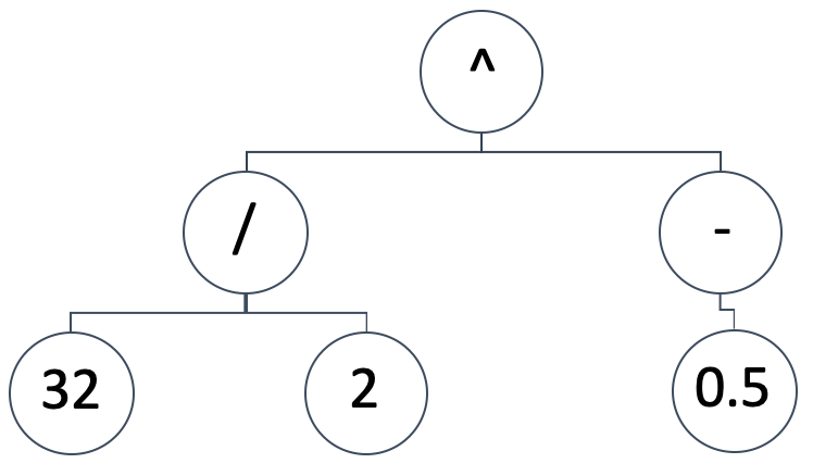
Would imply the mathematical expression:

(32/2) ^ (-0.5)

That would be equivalent to:0.25.Expression trees can take on a variety of forms and designs, we want to keep the foundational premise of SR, which is starting with a random and non-biased configuration. At the same time, we need to be able to run genetic optimizations on any size of an initially generated expression tree while being able to compare its result (or best-fit metric) to different sized expression trees.

To achieve this, we will run our genetic optimizations in ‘epochs’. Whereas epochs are common in machine learning lingo when batching training sessions like with neural networks, here we use the term to refer to different genetic optimization iterations where each run uses expression trees of the same size. Why do we maintain size within each epoch? Because genetic optimization uses cross-overs and if the expression trees are of different lengths, then this unnecessarily complicates the process. How then do we keep the initial expression trees random? By having each epoch represent a particular size of trees. This way we optimize across all epochs and compare all of them to the same benchmark or best-fit metric.

The fitness function measuring options available within MQL5’s vector/ matrix data types that we could use are regression and loss. These in-built functions will be applicable because we’ll be comparing the ideal output from the training data set as one vector against the outputs produced by the tested expression tree also in a vector format. So, the longer/ or larger the test data set, the larger our compared vectors. These large data sets will ten to imply that achieving the ideal zero best-fit value will be very difficult and therefore enough optimization generations need to be allowed for in each epoch.

In arriving at the best expression tree as based off of the best fit score, we will evaluate the expression trees from the longest (and therefore most complex) to the simplest and presumably easiest to ‘explain’. Our expression tree formats can take on a plethora of forms, however we will resort to the basic:

coeff, x-exponent, sign, coeff, x-exponent, sign, …

Where:

• Coeff represents the coefficient of x
• x-exponent is the power of x
• sign is an operator in the expression that could be -, +, *, or /

The last value to any expression will not be a sign because such a sign will not be connecting to anything, which means the signs will always be fewer than the x values in any expression. The size of such an expression will range from 1 where we only provide one x coefficient and exponent with no sign, up to 16 (16 is used here strictly for testing purposes). As eluded above, this maximum size directly correlates with the number of epochs to be used in the genetic optimization. This simply implies we start optimizing for the ideal expression with an expression tree that is 16 units long. These 16 units imply 15 signs, as mentioned above, and ‘each unit’ is simply an x coefficient and its x’s exponent.

So, in selecting the first random expression trees we will always follow the format of 2 random digit ‘nodes’ followed by a random sign ‘node’, if the expression tree is more than one unit long, and we are not terminating the expression i.e. we have a unit to follow. The listing that helps us achieve this is given below:

//+------------------------------------------------------------------+
// Get Expression Tree
//+------------------------------------------------------------------+
void CSignalSR::GetExpressionTree(int Size, string &ExpressionTree[])
{  if(Size < 1)
   {  return;
   }
   ArrayFree(ExpressionTree);
   ArrayResize(ExpressionTree, (2 * Size) + Size - 1);
   int _digit[];
   GetDigitNode(2 * Size, _digit);
   string _sign[];
   if(Size >= 2)
   {  GetSignNode(Size - 1, _sign);
   }
   int _di = 0, _si = 0;
   for(int i = 0; i < (2 * Size) + Size - 1; i += 3)
   {  ExpressionTree[i] = IntegerToString(_digit[_di]);
      ExpressionTree[i + 1] = IntegerToString(_digit[_di + 1]);
      _di += 2;
      if(Size >= 2 && _si < Size - 1)
      {  ExpressionTree[i + 2] = _sign[_si];
         _si ++;
      }
   }
}

Our function above starts by checking to ensure the size of the expression tree is at least one. If this test is passed, we then need to determine the actual array size of the tree. From above, we’ve seen that the trees follow the format coefficient, exponent, and then sign if applicable. This implies that given a size s, the total number of digit nodes in that tree will be 2 x s since each size unit must carry a coefficient and exponent value. These nodes are selected at random via the get digit node function, whose listing is shared below:

//+------------------------------------------------------------------+
// Get Digit
//+------------------------------------------------------------------+
void CSignalSR::GetDigitNode(int Count, int &Digit[])
{  ArrayFree(Digit);
   ArrayResize(Digit, Count);
   for(int i = 0; i < Count; i++)
   {  Digit[i] = __DIGIT_NODE[MathRand() % __DIGITS];
   }
}

Numbers are chosen at random from the static global digit node array. The sign nodes though will vary depending on whether, the size of the tree exceeds one. If we have a one sized tree then no sign would be applicable since this only leaves room for an x coefficient and its exponent. If we have more than one, then the number of sign nodes will be equivalent to the input size minus one. Our function for randomly selecting a sign to fill the sign slot in the expression is given below:

//+------------------------------------------------------------------+
// Get Sign
//+------------------------------------------------------------------+
void CSignalSR::GetSignNode(int Count, string &Sign[])
{  ArrayFree(Sign);
   ArrayResize(Sign, Count);
   for(int i = 0; i < Count; i++)
   {  Sign[i] = __SIGN_NODE[MathRand() % __SIGNS];
   }
}

Signs, like with the digit node array, are picked at random from the sign node array. This array though can take on a number of variants, but for brevity we are shortening it to accommodate just the ‘+’ and ‘-’ signs. The ‘*’ (multiplication) sign could be added to this, however the ‘/’ division sign was specifically omitted because we are not handling zero divides, which can be quite sticky once we start the genetic optimization and have to do crosses etc. The reader is free to explore this though provided the zero-divide issue is properly addressed as it could warp optimization results.

Once we have an initial population of random expression trees, we can begin the genetic optimization process for that particular epoch. Noteworthy as well is the simple struct we are using to store and access expression tree information. It essentially is a string matrix with added flexibility of resizing (features which should be provided by a standard data type like the matrix which handles doubles?). This is also listed below:

//+------------------------------------------------------------------+
//|
//+------------------------------------------------------------------+
struct Stree
{  string   tree[];

   Stree()
   {  ArrayFree(tree);
   };
   ~Stree() {};
};
struct Spopulation
{  Stree   population[];

   Spopulation() {};
   ~Spopulation() {};
};

We use this struct to create and track populations in each optimization generation. Each epoch uses a set number of generations to do its optimization. As already mentioned, the larger the test data set, the more optimization generations one would need. On the flip side, if the test data is too small, this may lead to expression trees that are derived mostly from white noise rather than the underlying patterns in the tested data sets, so a balance needs to be made.

Once we start our optimization on each generation we’d need to get the fitness of each tree and since we have multiple trees, these fitness scores are logged in a vector. Once we have this vector, the next step then becomes establishing a threshold for pruning this population, given that this tree gets refined and narrowed with each subsequent generation within a given epoch. We have called this threshold ‘_fit’ and it is based on an integer input parameter that acts as a percentile marker. The parameter ranges from 0 to 100.

We proceed to create another sample population from this initial population, where we select only the expression trees whose fitness is below or equal to the threshold. The function for computing our fitness score used above would have the listing given below:

//+------------------------------------------------------------------+
// Get Fitness
//+------------------------------------------------------------------+
double CSignalSR::GetFitness(matrix &XY, vector &Y, string &ExpressionTree[])
{  Y.Init(XY.Rows());
   for(int r = 0; r < int(XY.Rows()); r++)
   {  Y[r] = 0.0;
      string _sign = "";
      for(int i = 0; i < int(ExpressionTree.Size()); i += 3)
      {  double _yy = pow(XY[r][0], StringToDouble(ExpressionTree[i + 1]));
         _yy *= StringToDouble(ExpressionTree[i]);
         if(_sign == "+")
         {  Y[r] += _yy;
         }
         else if(_sign == "-")
         {  Y[r] -= _yy;
         }
         else if(_sign == "/" && _yy != 0.0)//un-handled
         {  Y[r] /= _yy;
         }
         else if(_sign == "*")
         {  Y[r] *= _yy;
         }
         else if(_sign == "")
         {  Y[r] = _yy;
         }
         if(i + 2 < int(ExpressionTree.Size()))
         {  _sign = ExpressionTree[i + 2];
         }
      }
   }
   return(Y.RegressionMetric(XY.Col(1), m_regressor));
   //return(_y.Loss(XY.Col(1),LOSS_MAE));
}

The get fitness function takes the input data set matrix ‘XY’, and focuses on the x column of the matrix (we are using single dimension data for both inputs and outputs) to work out the forecast value of the input expression tree. The input matrix has multiple rows of data so based on the x value at each row (the first column), a projection is made and all these projections, for each row are stored in a vector ‘Y’. After all the rows are processed, this vector ‘Y’ is compared to the actual values in the second column by using either the regression inbuilt function or the loss function. We choose regression, with root-mean-square error as the regression metric.

The magnitude of this value is the fitness value of the input expression tree. The smaller it is, the better the fit. Having got this value for each of the sampled population, we then need to first check that the sample size is even, if not we reduce the size by one. The size needs to be even because at the next stage we are crossing these trees and the generated crosses are added in pairs, and they should match the parent population (the samples) since we only reduce the population when sampling at each generation. The crossing of expression trees within the samples is done randomly by index selection. The function responsible for the crossing is listed below:

//+------------------------------------------------------------------+
// Set Crossover
//+------------------------------------------------------------------+
void CSignalSR::SetCrossover(string &ParentA[], string &ParentB[], string &ChildA[], string &ChildB[])
{  if(ParentA.Size() != ParentB.Size() || ParentB.Size() == 0)
   {  return;
   }
   int _length = int(ParentA.Size());
   ArrayResize(ChildA, _length);
   ArrayResize(ChildB, _length);
   int _cross = 0;
   if(_length > 1)
   {  _cross = rand() % (_length - 1) + 1;
   }
   for(int c = 0; c < _cross; c++)
   {  ChildA[c] = ParentA[c];
      ChildB[c] = ParentB[c];
   }
   for(int l = _cross; l < _length; l++)
   {  ChildA[l] = ParentB[l];
      ChildB[l] = ParentA[l];
   }
}

This function starts by checking that the two expression parents are of the same size and none of them is zero. If this is passed, then the two output child arrays are resized to match the parent lengths and then the cross point would be selected. This cross is also random and is only relevant when the parent size is more than one. Once the cross point is set, the two parents have their values swapped and outputted into the two child arrays. This where the matching lengths come in handy because, for instance, if they were to be different then extra code would be needed to handle (or avoid) cases where digits get swapped for signs. Clearly unnecessary complications when all sizes can be tested independently, in their own epoch, for the best fit.

Once we have finished the crossing, we may mutate the children. ‘May’ because we use a 5% probability threshold to do these mutations, as they are not guaranteed but are typically part of the genetic optimization process. We then copy this new crossed population to over write our starting population from which we had sampled at the start and as a marker we log the best fit score of the best expression tree from this newly crossed population. We use the logged score not only to determine the best fit tree, but also in some rare cases to halt the optimization in the even that we get a zero value.

Custom Signal Class

In developing the signal class, our main steps do not differ a lot from what we’ve done in previous custom signal classes through these series. Firstly, we’d need to prepare the data set for our model. This is the data that fills our ‘XY’ input matrix for the function looked at above of get fitness. It is also an input to the function that integrates all the steps we’ve outlined above, called ‘get best tree’. The source code to this function is given below:

//+------------------------------------------------------------------+
// Get Best Fit
//+------------------------------------------------------------------+
void CSignalSR::GetBestTree(matrix &XY, vector &Y, string &BestTree[])
{  double _best_fit = DBL_MAX;
   for(int e = 1 + m_epochs; e >= 1; e--)
   {  Spopulation _p;
      ArrayResize(_p.population, m_population);
      int _e_size = 2 * e;
      for(int p = 0; p < m_population; p++)
      {  string _tree[];
         GetExpressionTree(e, _tree);
         _e_size = int(_tree.Size());
         ArrayResize(_p.population[p].tree, _e_size);
         for(int ee = 0; ee < _e_size; ee++)
         {  _p.population[p].tree[ee] = _tree[ee];
         }
      }
      for(int g = 0; g < m_generations; g++)
      {  vector _fitness;
         _fitness.Init(int(_p.population.Size()));
         for(int p = 0; p < int(_p.population.Size()); p++)
         {  _fitness[p] = GetFitness(XY, Y, _p.population[p].tree);
         }
         double _fit = _fitness.Percentile(m_fitness);
         Spopulation _s;
         int _samples = 0;
         for(int p = 0; p < int(_p.population.Size()); p++)
         {  if(_fitness[p] <= _fit)
            {  _samples++;
               ArrayResize(_s.population, _samples);
               ArrayResize(_s.population[_samples - 1].tree, _e_size);
               for(int ee = 0; ee < _e_size; ee++)
               {  _s.population[_samples - 1].tree[ee] = _p.population[p].tree[ee];
               }
            }
         }
         if(_samples % 2 == 1)
         {  _samples--;
            ArrayResize(_s.population, _samples);
         }
         if(_samples == 0)
         {  break;
         }
         Spopulation _g;
         ArrayResize(_g.population, _samples);
         for(int s = 0; s < _samples - 1; s += 2)
         {  int _a  = rand() % _samples;
            int _b  = rand() % _samples;
            SetCrossover(_s.population[_a].tree, _s.population[_b].tree, _g.population[s].tree, _g.population[s + 1].tree);
            if (rand() % 100 < 5)   // 5% chance
            {  SetMutation(_g.population[s].tree);
            }
            if (rand() % 100 < 5)
            {  SetMutation(_g.population[s + 1].tree);
            }
         }
         // Replace old population
         ArrayResize(_p.population, _samples);
         for(int s = 0; s < _samples; s ++)
         {  for(int ee = 0; ee < _e_size; ee++)
            {  _p.population[s].tree[ee] = _g.population[s].tree[ee];
            }
         }
         // Print best individual
         for(int s = 0; s < _samples; s ++)
         {  _fit = GetFitness(XY, Y, _p.population[s].tree);
            if (_fit < _best_fit)
            {  _best_fit = _fit;
               ArrayCopy(BestTree,_p.population[s].tree);
            }
         }
      }
   }
}

The input matrix pairs single dimension x values and single dimension y values. Independent variables and dependent variables. Multidimensionality could also be accommodated with the ‘Y’ input vector being transformed into a matrix and an expression tree for each x value in the input vector, for each y value in the output vector. These expression trees would also have to be in a matrix or higher dimension storage format.

We are using single dimensions, though, and our data row simply consists of consecutive close prices. So, on the top or most recent data row, we’d have the penultimate close price as our x value and the current close price as our y. The preparations and the filling of our ‘XY’ matrix with this data is handled by the source code below:

//+------------------------------------------------------------------+
//| "Voting" that price will grow.                                   |
//+------------------------------------------------------------------+
int CSignalSR::LongCondition(void)
{  int result = 0;
   m_close.Refresh(-1);
   matrix _xy;
   _xy.Init(m_data_set, 2);
   for(int i = 0; i < m_data_set; i++)
   {  _xy[i][0] = m_close.GetData(StartIndex()+i+1);
      _xy[i][1] = m_close.GetData(StartIndex()+i);
   }

...

   return(result);
}

Once our data preparation is done, it is a good idea to be clear about the fitness evaluation method to be used in our model. We are opting for regression as opposed to loss, buteven within regression there are quite a few metrics to select from. To therefore allow an optimal selection, the type of regression metric to be used is an input parameter, that could be optimized to better suite tested data sets. Our default value though is the common root-mean-square-error.

The implementation of the genetic algorithm is handled by the get best tree function, whose source code is already listed above. It returns a number of outputs chiefs among which is the best expression tree. With this tree we can process the current close price as an input (x value) to get our next close (y value), using the get fitness function as it also returns more than just the fitness of a queried expression since the input ‘Y’ vector contains our target forecast. This is handled in the code below:

//+------------------------------------------------------------------+
//| "Voting" that price will grow.                                   |
//+------------------------------------------------------------------+
int CSignalSR::LongCondition(void)
{ 
        ...

   vector _y;
   string _best_fit[];
   GetBestTree(_xy, _y, _best_fit);

        ...

   return(result);
}

With an indicative next close price obtained, the next step is to convert this price into a usable signal for the Expert Advisor. The forecast values are often only indicative of a rise or fall, but their absolute value is out of range when compared to the recent close price values. This means we would need to normalize them before they can be used. The normalization and signal generation are done in our code below:

//+------------------------------------------------------------------+
//| "Voting" that price will grow.                                   |
//+------------------------------------------------------------------+
int CSignalSR::LongCondition(void)
{  int result = 0;
   
        ...

   double _cond = (_y[0]-m_close.GetData(StartIndex()))/fmax(fabs(_y[0]),m_close.GetData(StartIndex()));
   _cond *= 100.0;
   //printf(__FUNCSIG__ + " cond: %.2f", _cond);
   //return(result);
   if(_cond > 0.0)
   {  result = int(fabs(_cond));
   }
   return(result);
}

The integer output of both long and short conditions in a standard Expert signal class has to be in the range 0 – 100 and this is what we are converting our signal to in the above code.

The long condition function and short condition function are mirrors of each other, and the assembly of signal classes into Expert Advisors is covered in articles here and here.

Back testing and Optimization

On performing a test run with some of the ‘best settings’ of the assembled Expert Advisor, we get the following report and equity curve:

For any given settings, because expression trees are got from random selection and are crossed and mutated also randomly any particular test run is unlikely to replicate its results exactly however, and interestingly if a test run is profitable, then subsequent runs with the same settings will have different performance statistics but, on the whole, will also be profitable. Our testing is performed for the year 2022, on the pair EUR JPY on the 4-hour time frame. As always, we run tests without price targets for SL or TP as this could help better identify ideal Expert settings.

Conclusion

To recap, we’ve introduced symbolic regression as a model that could be used in a custom instance of an Expert signal class to weigh long and short conditions. We used a very modest data set in this analysis, as both the input and output values of the model were unidimensional. This doesn’t mean the model cannot be expanded to accommodate multidimensional data sets. In addition, the genetic optimization nature of the model’s algorithm makes it tricky to obtain identical results from each test run. This implies Expert Advisors based on this model should be used on fairly large time frames and in tandem with other trade signals so that they can act as a confirmation to already independently generated signals.