Combinatorics and probability for trading (Part V): Curve analysis

MetaTrader 5 — Trading | 8 February 2022, 11:20

8 591

Evgeniy Ilin

Introduction

I continue preparing the basis for building multi-stage and scalable trading systems. Within the framework of this article, I want to show how you can use the developments from the previous articles to get closer to the broader possibilities for describing the trading process. This will assist in evaluating the strategy from those sides, which are not covered by other methods of analysis. In this article, I explored the possibilities of transforming complex, multi-state samples to simple double-state ones. This analysis was done in a research style.

Useful forms to simplify data

Suppose there is a strategy with many trades that go one after another, without overlapping, that is, a new order is opened strictly after the previous one has closed. If we need to evaluate the probability of winning or losing and to measure the average time required to achieve the profit or loss, we will see that the orders can have a very large number of different states (they are closed with different results).

In order to be able to apply fractal formulas to such strategies, we first need to convert these strategies to the cases that can be considered within the frameworks of fractals. To implement this, we need to represent our strategy as an order with equidistant stop-levels, which has the probability of a step up and a step down, just like in our fractal. Then, we can apply the fractal formulas. Also, a step up and a step down can have different lifetime.

In order to reduce any strategy to one of the types that can be described in the framework of fractal formulas, which we found in the previous article, we first need to determine which values must be known in order to be able to apply the fractal formulas. Everything is pretty simple here:

P[1] – the probability of the step up
T[1] – average up step formation time
T[2] – average down step formation time

First, we need to consider the limit values when the number of steps tends to infinity:

(P[1] * T[1] + (1 -P[1])*T[2]) * n = T(n)
(P[1] * Pr - (1 -P[1])*Pr) * n = P(n)

In order to better understand the above expressions, it is necessary to write two limits:

Lim(n --> +infinity)[P/P0(n)] = 1
Lim(n --> +infinity)[T/T0(n)] = 1

The limits say that if we conduct the same experiments in the amount of "n", or trades, we will always get different total time which all the elementary experiments included in the main general experiment took. Also, we will always get different positions of the final trading balance. On the other hand, it is intuitively clear that with an infinite number of experiments, the real value will tend to the limit. We can prove this fact using random number generators.

n - emulated number of steps
1-P[1] – probability of the step down
T0(n) – real amount of time spent on "n" steps
P0(n) – real shift of the balance or price for "n" steps
T(n) - the limit amount of time spent on "n" steps
P(n) – the limit shift for "n" steps

This logic results in two equations which however too many unknowns. This is not surprising as this is only the beginning. But these equations describe only the derived system (the one we need to get). The equations for the source system are similar:

(P*[1] * T[1] + P*[2])*T*[2] + … + P*[N])*T*[N] ) * m = T(m)
(P*[1] * Pr*[1] + P*[2]*Pr*[2] + … + P*[N1]*Pr*[N1]) * m - (P*[N2] * Pr*[N1] + P*[N1+1]*Pr*[N1+1] + … + P*[N2]*Pr*[N2]) * m = P(m)

P*[1] + P[*2] + … + P*[N2] = 1 – the probabilities form a complete group

The limits are also the same, and they show the same values:

Lim(m --> +infinity)[P/P0(m)] = 1
Lim(m --> +infinity)[T/T0(m)] = 1

The variables that are used here are described below:

m – emulated number of steps
T0(m) – real amount of time spent on "m" steps
P0(m) – real shift of the balance or price for "m" steps
T(m) - real amount of time spent on "m" steps
P(m) – real shift for "m" steps
T = Lim(m --> +infinity) [ T(m) ] – limit time
N1 – the number of trade outcomes with positive profit and their counter
N2 – N1 + 1 – number of trade outcomes with negative profit (N2 is their counter)

Based on the source system, we need to create a new, simpler one, composed of a more complex one. The only difference is that we know all the parameters of the original system. The known values are shown with asterisks * postfixes.

If we equate the second and first equations from both systems, we can eliminate the variables P and T:

(P[1] * T[1] + (1 -P[1])*T[2]) * n = (P*[1] * T[1] + P*[2])*T*[2] + … + P*[N])*T*[N] ) * m
(P[1] * Pr - (1 -P[1])*Pr) * n = (P*[1] * Pr*[1] + P*[2]*Pr*[2] + … + P*[N1]*Pr*[N1]) * m - (P*[N2] * Pr*[N1] + P*[N1+1]*Pr*[N1+1] + … + P*[N2]*Pr*[N2]) * m

As a result, we lost two equations, but at the same time we eliminated two unknowns, which were not necessary. As a result of these transformations, we have one equation, in which the following quantities are unknown:

P[1] – the probability of the step up (stop)
T[1] – the average lifetime of the step up
T[2] – the average lifetime of the step down

These two equations have a similar structure:

A1*n = A2*m
B1*n = B2*m

The structure indicates that one of the variables, "n" or "m", can be excluded to eliminate one of the equations. For this, we need to express one of the values, for example from the first equation:

m = ( (P[1] * T[1] + (1 -P[1])*T[2]) / (P*[1] * T[1] + P*[2])*T*[2] + … + P*[N])*T*[N] ) )* n

Then, let's substitute the expression to the second equation and see the result:

(P[1] * Pr - (1 -P[1])*Pr) * n = (P*[1] * Pr*[1] + P*[2]*Pr*[2] + … + P*[N1]*Pr*[N1]) * ( (P[1] * T[1] + (1 -P[1])*T[2]) / (P*[1] * T[1] + P*[2])*T*[2] + … + P*[N])*T*[N] ) ) * n - (P*[N2] * Pr*[N1] + P*[N1+1]*Pr*[N1+1] + … + P*[N2]*Pr*[N2]) * ( (P[1] * T[1] + (1 -P[1])*T[2]) / (P*[1] * T[1] + P*[2])*T*[2] + … + P*[N])*T*[N] ) ) * n

Now, both parts of the equation are multiplied by "n". So, by dividing them by "n", we will get an equation depending only on the required values:

(P[1] * Pr - (1 -P[1])*Pr) = (P*[1] * Pr*[1] + P*[2]*Pr*[2] + … + P*[N1]*Pr*[N1]) * ( (P[1] * T[1] + (1 -P[1])*T[2]) / (P*[1] * T[1] + P*[2])*T*[2] + … + P*[N])*T*[N] ) ) - (P*[N2] * Pr*[N1] + P*[N1+1]*Pr*[N1+1] + … + P*[N2]*Pr*[N2]) * ( (P[1] * T[1] + (1 -P[1])*T[2]) / (P*[1] * T[1] + P*[2])*T*[2] + … + P*[N])*T*[N] ) )

Value "Pr" shall be considered free, as the number of systems to which all can be reduced is infinite. We can set absolutely any step size, given that the steps up and steps down are equal in absolute values. Other values will be determined by solving a system of equations. So far, the system has only one equation. We need two more equations, which can be obtained using the equations obtained in the previous section.

First of all, the system should have an identical probability of upper corridor border and lower bound crossing. Also, it should have an identical average time to crossing one of the bounds. These two requirements will give us the two missing equations. Let's start with determining the average time till crossing of the corridor bound. The average time till one of the bounds is crossed is determined by the average number of steps up and down. Taking into account the results of the previous article, we can write the following:

T[U,D] = (S[U,u] * T[1] + S[U,d] * T[2]) * P[U] + (S[D,u] * T[1] + S[D,d] * T[2]) * ( 1 – P[U] )

This equation indicates that the average time to crossing one of the bounds depends on the average number of steps when one of the bounds is crossed, as well as the on the probability of crossing. This criterion will provide another possible equation with which we can create a system of equations that will allow us to transform a complex trading system to a simpler one. This equation can be split into two other equations:

T[U] = S[U,u] * T[1] + S[U,d] * T[2]
T[D] = S[D,u] * T[1] + S[D,d] * T[2]

We will need these equations later. All these values are calculated based on the mathematical model obtained in the previous article:

S[U,u], S[U,d], S[D,u], S[D,d], P[U] = f(n,m,p) – all these values are functions of "n,m,p"
n = B[U]/ Pr - in turn, "n" can be expressed in terms of the distance to the upper bound and the step "Pr"
m = B[D]/ Pr – in turn, "m" can be expressed in terms of the distance to the upper bound and the step "Pr"
Pr – selected step
B[U] – distance to upper bound
B[D] – distance to lower bound

Basics of the resulting transformation method

As an example, we can take a random strategy and convert it to the required equivalent. I have created one of the variants of transforming a complex multidimensional system into a simpler, two-dimensional one. I will try to provide a step-by-step description of this process. Before proceeding to description, I implemented the idea and tested the method performance. The program is attached to the article. In my program I used slightly different yet equally effective formulas. It is based on the mathematical model obtained in the previous article. Using it, we can obtain the following values:

P[U], S[U,u], S[U,d], S[D,u], S[D,d]

From average steps, we can get the average time before the upper or lower border is crossed. The purpose might not be quite clear for now. It should become clearer with further explanation. To transform a multi-state strategy into a simpler one, we should first generate the relevant strategies. I have created a random number-based strategy generator. For convenience, I took five randomly generated strategies. They are as follows:

Five random strategies

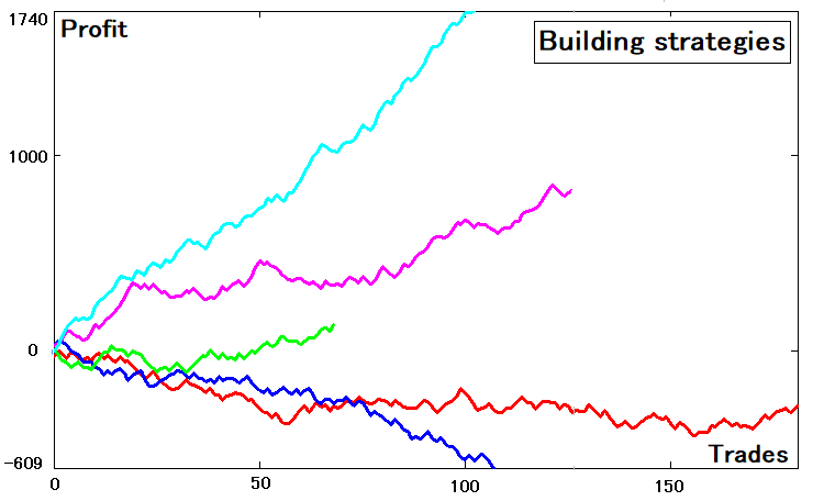
These strategies have different Expected Payoff metrics, different number of deals and parameters. Some of the curves are losing, but this is ok, as it is still a curve, though its parameters might not be quite good.

Now to the point. The figure shows the balance graphs that depend on the trade number, similar to the strategy tester graphs. According to it, there is a certain array of balances for each curve:

B[i] , i = 0…N
N – number of trades

This array can be obtained from the array with order parameters. I assume that the container with the order data only contains the order profit or loss value, as well its lifetime:

Pr[i], T[i]

Let's assume that other parameters are not available. I think this is correct, because when we want to analyze any backtest or signal, this data is usually unavailable to us, since normally no one saves this data. More often, users check the recovery factor, maximum drawdown and similar metrics. The only trading data that is always saved is:

Profit
Order opening time
Order closing time

Of course, the unavailability of some data will affect the accuracy, but there is nothing to do with that. Now, let's see how to get an array with balances from an array with profits:

B[i] = B[i-1] + Pr[i] if i > 0
B[i] = 0 else

In order to enable the analysis of the obtained strategies against time, we need to create a similar time array:

TL[i] = TL[i-1] + T[i] if i > 0
TL[i] = 0 else

After determining the abscissas and ordinates of all such curves, we can plot them. You will see the differences, since we these are functions with dependence not on the trade number, but on time:

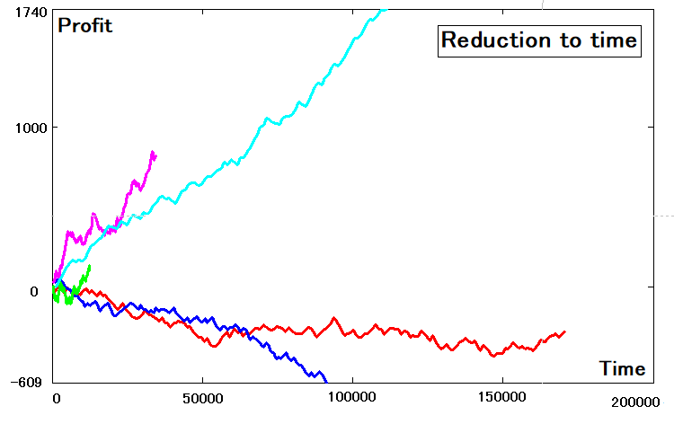
5 strategies reduced to the time argument

Defining reducibility criteria

We can further work with the obtained data. Now, we can determine the criteria according to which we will check if curves match two profit states. From the point of view of representation relative to time, three quantities will be enough:

P[U] – the probability of crossing the upper bound
T[U] – the average time till the upper bound is reached
T[D] – the average time till the lower bound is reached

The second and the third values can be calculated as follows:

T[U] = S[U,u] * T[u] + S[U,d] * T[d]
T[D] = S[D,u] * T[u] + S[D,d] * T[d]

As for P[U], this value is provided by the mathematical model which we obtained in the previous article And, as you remember, "P[D] = 1 – P[U]". Thus, based on the five values provided by the mathematical model, we can for the required three values described above. As for these two equations, we have obtained them earlier, but here I changed the notation for time for convenience.

These values are calculable. In order to reduce them to something, we need to somehow obtain their real value based on what we have. Then, we need to find such parameters of the desired, equivalent two-state curve that all the three parameters would be very similar to real values. This is how we get the criteria. First, let's introduce the notation for the known values:

P*[U] – the real probability of crossing the bounds of the selected corridor
T*[U] – the real average time till the upper bound is crossed
T*[D] – the real average time till the lower bound is crossed

The deviation of real and calculated values can be measured either in relative terms or as a percentage. If measured in percentage, the criteria will be as follows:

KPU = ( | P[U] – P*[U] | / ( P[U] + P*[U] ) ) * 100 %
KTU = ( | T[U] – T*[U] | / ( T[U] + T*[U] ) ) * 100 %
KTD = ( | T[D] – T*[D] | / ( T[D] + T*[D] ) ) * 100 %

Defining criteria for comparison with the source system

The best system is the one that has a minimum of all these values. Now, in order to be able to obtain the calculated values, we first need to determine the size of corridor, according to which we will determine the real probability and real time till breakout. This idea can be visualized as follows:

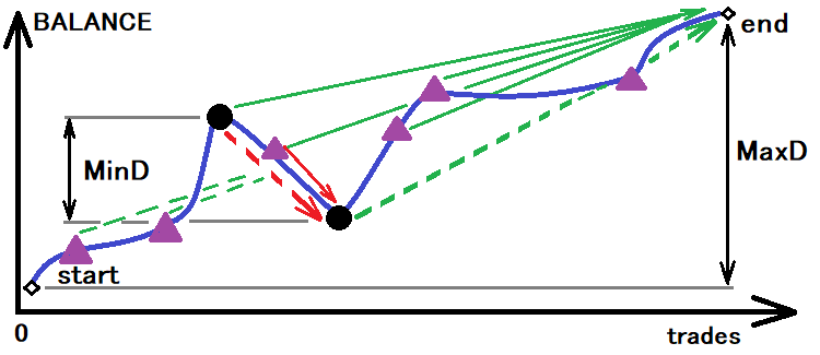
Determining the minimum corridor value

The figure shows an example of determining such a corridor for a profitable strategy. The purple triangles symbolize another check point for possible up and down moves. The desired minimum movement is between the black dots. If we take the maximum movement that happened in the available period as the basis, then the probability P[U] will be one. Obviously, this is the most incorrect choice. Because we need the minimum value which guarantees the crossing of both the lower and the upper bounds.

Assessing a possible corridor for calculating the required values

However, even this is not enough. If we use this value as the basis, we will have only one touch of the lower bound, which is also not accurate. Personally, I used the value of the corridor three times less than the given minimum. With a sufficient sample of bound touches, this value will be enough. Now that we have determined the corridor size, we can split this corridor. If we assume that the corridor itself is a step, then:

n, m = 1
p = P[U]
Pr * n = Pr * m = 1/3 * MinD – half of the corridor width
Pr = ( 1/3 * MinD ) / n = ( 1/3 * MinD ) / m – step module
T[U,u] = T[U]
T[D,d] = T[D]
T[U,d] = 0
T[D,u] = 0

This variant can also be used in case you have a very large trading sample. The advantage of this approach is that we do not need to use a mathematical model for splitting the corridor, because in this case our entire corridor is one step. But in my calculations I used a mathematical model as an example. When using this approach, it is necessary to find the following ranges of parameters for selection:

p = p1 … p2
N = m = nm1 …. nm2

In my example, I used the following ranges:

p1 = 0.4, p2 = 0.6, nm1 = 1, nm2 = 3

Of course, you can use wider ranges. Optionally, one of the ranges can be widened, while the other one used as is. For example, if we increase "nm2", then the method can cover a wider range of various strategies. If the mathematical model cannot handle the next variant, then we can switch to the one without the math model.

Defining the probability and average time till the crossing of the upper border of the corridor

After successfully finding all the above values, we will only get the probability “p” for a step up. We can then use this value as a basis for finding the average border crossing time. This can be visualized by a slight transformation of the above image above:

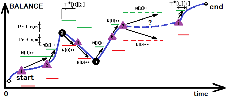
Determining the probability of corridor crossing and the average time

The figure shows the process of summing up upper and lower crossings for the corridor which size was determined as a result of the previous transformation. Along with the summation of these crossing, we calculate time required for intersection. In one operation, we can determine all the quantities with an asterisk that we need:

N[U] – the number of intersections of the upper border of the corridor
N[D] – the number of intersections of the lower border of the corridor
T[U][i] – array with the time till the upper border is crossed
T[D][i] – array with the time till the lower border is crossed

Using this data, let's calculate the probability of upper border crossing and the average time to cross the upper and lower borders:

P*[U] = N[U]/ ( N[U] + N[D] )
T*[U] = Summ( 0…i ) [ T[U][i] ] / N[U]
T*[D] = Summ( 0…i ) [ T[D][i] ] / N[D]

We have found all the values, to which our two-dimensional equivalent should be reduced. Now, we need to define where to start the search. To do this, we need to determine which of these values has the highest priority in terms of accuracy. I have chosen the probability of crossing the upper border as an example. This approach reduces the computational requirements for the analysis. If we choose to select three values in three intervals, then we would get three degrees of freedom, which would increase the calculation time. Sometimes, the calculation time would be unreal. Instead, I started with the probability of a step up, and then proceeded to the average time of steps up and down.

I want to remind you that there are many steps in the corridor and the time to crossing is not the time of steps. Also, the probability of a step in a certain direction is not the probability of bound crossing. The only exception is the situation n=m=1 described at the beginning.

As a result, we get the following step characteristics:

p – probability of a step up
T[u] – average duration of a step up
T[d] – average duration of a step down
Pr – step modulus in profit values

Estimating the efficiency of a simple transformation

Suppose we have found all the parameters of the steps. How to evaluate the general efficiency of such a transformation operation? To evaluate the efficiency, we can draw straight lines to which the strategies are reduced. The slope of the lines can be defined as follows:

K = EndProfit / EndTime – line slope coefficient
P0 = K * t – line equation

This is how it will look like:

Ideal case

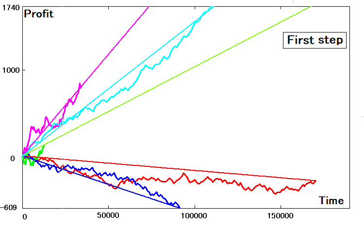
If the parameters of the two-dimensional curves are ideal, then their similar straight lines will have exactly the same slope and will touch the balance curves at the end points. I think it's clear that most such a coincidence can never happen. To find the slope coefficient for this equivalent, we can use the data found for the step:

MP = p * Pr – (1-p) * Pr – math expectation of an upward shift for any step
MT = p * T[u] + (1-p) * T[d] - math expectation of the time spent on the formation of any step
K = MP / MT – line slope coefficient.

I used the same program for calculation and every time I got a similar picture:

Close to real case

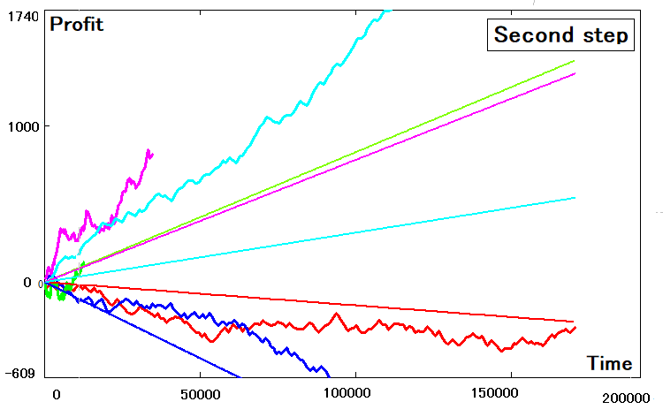
Not all the strategies could be correctly transformed into a two-dimensional equivalent. Some of them have clear deviations. The deviations are connected with the following reasons:

Error in calculating values with an asterisk
Imperfection of the two-dimensional model (less flexible model)
Finiteness of the possible number of search attempts (and the limited computing power)

Taking into account all these facts, we can adjust the average step time, so that at least the slope coefficients of the original and derived models are equal. Of course, such transformations would affect the deviations of the criteria we are reducing, but there is no other solution. I think the main criterion is the line slope coefficient, because if the number of trades tends to infinity, the original and the derived strategies should merge into one line. If this does not happen, then there is not much sense in such a transformation. Perhaps, this is all connected not with the method of transformation, but with the hidden possibilities which are not quite clear now.

Final adjustment and simulation

In order to make such a transformation, we can use a proportion. Before creating the curves, we had the arrays TL[i], B[i], which are equivalent to the time since the beginning of the curve will the analyzed order or segment, we can take the last elements of the array and write the following:

K = B[n] / TL[n]
N – the index of the last element of the balances array (final balance)

For the straight lines obtained at the previous step we can also calculate such a coefficient. It was already calculated earlier:

K1 = MP / MT

These coefficients are not equal, so a correction is needed. This can be done as follows:

K = MP / ( KT * MT )
KT – correction coefficient

Now we need to add this coefficient inside the mathematical expectation so that the mathematical expectation does not change its meaning. This can be done like this:

MTK = MT * KT = p * (T[u]* KT) + (1-p) * (T[d]* KT)

As you can see, new corrected time values are now included in brackets. They can be calculated as follows:

Tn[u] = T[u]* KT
Tn[d] = T[d]* KT

This is our corrected time of a step up and a step down. To calculate the correction coefficient, we equate coefficient calculation expressions:

B[n] / TL[n] = MP / ( KT * MT )

Having solved the equation relative to KT, we obtain an expression for calculating this value:

KT = ( MP / MT ) / ( B[n] / TL[n] ) = ( MP * TL[n] ) / ( MT * B[n] )

All we need to do is to adjust the average time of a step up and a step down. After that, the conversion process can be considered completed. As a result, we get a set of four values which completely describe our strategy — instead of huge arrays that describe more than two states:

p – probability of a step up
Pr – step module
T[u] – average up step formation time
T[d] – average down step formation time

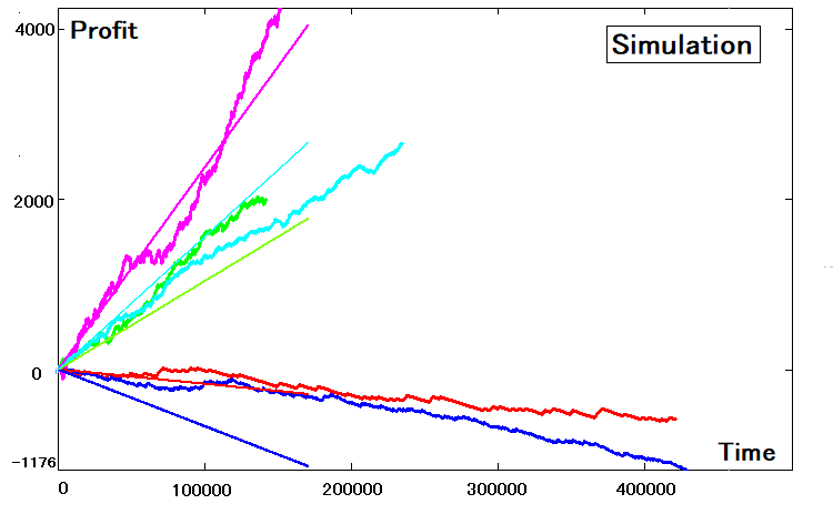
These four parameters are enough to recreate the strategy by simulation. Now this software is available to us, regardless of the market and time. The simulation for our five strategies is as follows:

Simulation

Here we use straight lines from the first step. These lines are drawn from zero to the end of the real trade curve. As you can see, simulation is very close to the lines, which confirms the correctness of transformations. The only exception is the blue line. I guess there are some minor flaws in my algorithm, which can be fixed with a little time.

Summary

The model studying process generated interesting ideas. Originally, when studying two-dimensional schemes and multi-state schemes, I only wanted to obtain a simplified description for complex systems. As a result of this analysis, we have received much more valuable and simple conclusions. The details are hard to describe in the article, as they imply too many technical nuances. In a nutshell, this study has yielded:

Research chart

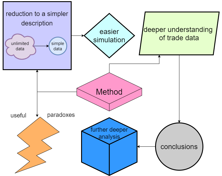
All the advantages can be presented in a list:

Many multi-state systems can be converted to two-state systems (and therefore the process of n to m states is also possible)
The conversion process can be used as a trading data compression mechanism
The converted data can be fed back through the simulation, which also simplifies the simulation (because only two states need to be simulated)
A deeper understanding of the probabilistic processes within pricing allows for individual useful conclusions.
Based on the information received, we can proceed to a deeper analysis of the trading process
We have obtained some useful features for trading — for now I categorize them as paradoxes

Of course, the main idea of the series is the construction of simple and useful mathematics which will directly allow the creation of ultra-stable and multi-currency systems based on probability theory. So far, the obtained information serves as a good foundation for building a monolith solution.

Also, I would like to mention the paradoxes that we revealed in the course of the study. In the first transformation stage, we obtained discrepancies which were expressed in a different slope of the equivalent straight line. I think these discrepancies can be used to convert random trading into non-random trading, or to provide various trading signal amplifiers.

In other words, they might be useful in converting some zero strategies into strategies with the positive PF if we apply transformations for converting multi-state systems into two-state ones, which can further be handled using other methods aimed at improving their quality. So far, these thoughts are too vague and scattered, but ultimately they will be converted into ideas. I consider this the main result of the study, which we will use later when creating an Expert Advisor.

Conclusion

In this article, I tried not to dive too deep into detail. Of course, this topic involves mathematics. However, given the experience of previous articles, I see that generalized information is more useful than details. If you want to study all the details of the method, please use the program attached below — I conducted research in this program. I did not describe all the algorithms used, because they imply a lot of boring mathematics, basically related to data arrays and matrices. I think if anyone wishes to create something similar, they will stick to their own logic, but may use the presented program as a starting point.

If you do not want to go analyze it deeper, I suggest testing different strategies to see how they will be converted. As for future ideas, I think we will gradually move on to creating a sound self-adapting algorithm that will be able to surpass neural networks both in quality and in stability. I already have some ideas. But first, we need to complete the foundation.

References

Translated from Russian by MetaQuotes Ltd.
Original article: https://www.mql5.com/ru/articles/10071

Attached files |

Download ZIP

Research_program.zip (1145.88 KB)

Warning: All rights to these materials are reserved by MetaQuotes Ltd. Copying or reprinting of these materials in whole or in part is prohibited.