Combinatorics and probability for trading (Part IV): Bernoulli Logic

Contents

• Introduction
• The importance of correct data representation in analysis
• Double states
• Multiple states
• Software implementation of multiple states
• Conclusion
• References

Introduction

In the previous articles within this series, I described fractals as a tool for describing markets and, in particular, pricing. This model perfectly describes the market — this has been confirmed through calculations and simulations. The original purpose was not only to describe the simplest pricing forms, but also to enable further description of any vector series which have a set of parameters similar to the pricing set of parameters. Well, in the general case, it turns out that a trade is also a piece of market, which is characterized by a duration in time and a probability of appearing in the trading process. Arbitrary curves can be created both from prices and from trades. For prices, this curve is the price history, while for trades it is the trading history.

The case with the price is much clearer, as all members in such a series clearly follow one another. Of course, it is possible to creates such price series that will overlap each other, but this analysis would be absolutely useless, as there would be no practical benefit from such an analysis. The case of backtests, or trading history, is more complicated. When studying these processes, I came to the conclusion that there is a much easier and more correct path to profitable and stable trading — through the analysis of trading history or backtests. There will be a final article describing one of these approaches, but it's too early for it as for now.

The importance of correct data representation in analysis

If we consider the analysis of the possibilities of describing trading history and backtests in the language of mathematics, first we need to understand the purpose and possible outcome of such analysis. Is there any added value in such an analysis? In fact, it is impossible to give a clear answer right away. But there is an answer, which can gradually lead to simple and working solutions. However, we should delve into more details first. Given the experience of previous articles, I was interested in the following questions:

1. Is it possible to reduce any strategy to a fractal description of trading?
2. If it is possible, where would it be useful?
3. If it is not always possible, what are the conditions for reducibility?
4. If the reducibility conditions are met, develop the reduction algorithm
5. Consider other options to describe the strategy. Generalization

The answers to all these questions are as follows. It is possible to reduce some strategies to fractal description. I have developed this algorithm and I will describe it further. It is suitable for other purposes as well, as it is a universal fractal. Now, let's think and try to answer the following question: What is the trading history in the language of random numbers and probability theory? The answer is simple: it is a set of isolated entities or vectors, the occurrence of which in a certain period of time has a certain probability and the time utilization factor. The main characteristic of each such entity is the probability of its occurrence. The time utilization factor is an auxiliary value that helps determine how much of the available time is being used for trading. The following figure may assist in understanding the idea:

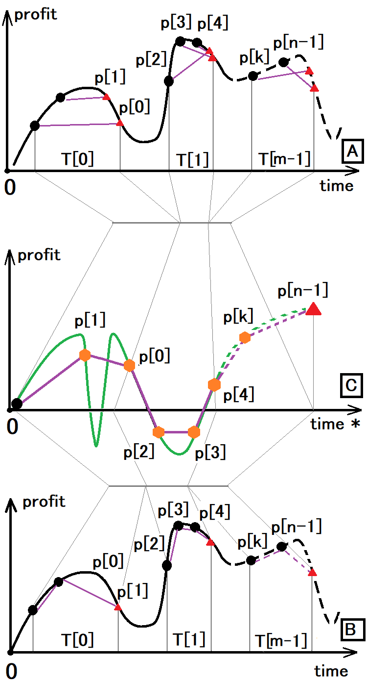
The following symbols are used in the figure:

1. Black dot - the beginning of the trade
2. Red triangle - the end of the trade
3. Orange hexagon - both the end of the previous trade and the beginning of the next one
4. T[i] – time of a relevant trading window
5. P[i] – profit or loss of a relevant trade
6. n – number of trades
7. m – number of trading windows

The figure shows three charts to demonstrate that options A and B can be reduced to option C. Now let's see what these options are:

1. Option A is how we see arbitrary trading using all possible tricks, money management, etc.
2. Option B is the same but considering that only one order can be open at a time.
3. Option C is how we see trading either in the Signals service or in the backtest.

Here option C is the most informative one and in most cases we rely on this representation of trading. Furthermore, absolutely any strategy can be reduced to this type because the equity line is the main characteristic of any backtest or trading signal. This line reflects real profit or loss as at the current moment.

The analysis of the equity line of an arbitrary strategy would show that deal opening and closing points can be located in absolutely arbitrary positions if the line remains unchanged. This means that a trading strategy can be represented in a huge number of different ways and all these ways will be equivalent as their equity lines are equivalent. Therefore, there is no point in searching for all equivalent options. What is the purpose of finding them?

A strategy of type B can be easily converted to type C, because we only need to glue together time intervals in the same order as they occur. Actually, this is exactly what the tester and the signal service do. Situation is different if you try to convert type A to C. In order to implement this conversion, we first need to reduce A to type B, and then the result can be reduced to type C. Now you know how the strategy tester and the Signals service work.

This transformation by itself does not carry any practical value for trading. However, it can assist in understanding deeper things. For example, we can conclude that there are the following types of strategies:

1. Described by two states
2. Described by multiple states
3. Described by an infinite number of states

In this article, I will show you description examples for the first two types of strategies. The third type is more complex and requires a separate article. I will return to this idea in due time. Anyway, before considering the third type of strategies, it is necessary to understand the first two. These two types will prepare our minds before we proceed with the third, general strategy type.

Double states

The fractals described in previous articles actually represent a two-state model. Here states are upward and downward movements. If we apply the model to the trading balance line rather than pricing, this model will work in exactly the same way. The model is based on the Bernoulli scheme. The Bernoulli scheme describes the simplest fractal with two states:

• P[k] = C(n,k)*Pow(p,k)*Pow(q,n-k)   — Bernoulli formula (P[k] is the probability of a specific combination)
• p is the probability of state “1” as an outcome of a single experiment
• q is the probability of state “2” as an outcome of a single experiment

These formulas can calculate the probability that after “n” steps we will have a balance curve or any other curve which will have “k” first states and “n-k” second states. these do not have to be trade profits. These states can symbolize any parameter vector in which we see uniqueness. The sum of all probabilities of a particular combination must form a complete group, which means that the sum of all such probabilities must be equal to one. This symbolizes the fact that in “n” steps one of such combinations must necessarily appear:

• Summ(0...k…n)[ P[k] ] = 1

In this case, we are interested in using these things to describe either pricing or backtests and signals. Imagine that our strategy consists of trades that are closed by equidistant stop levels. At the same, time we know that it is impossible to calculate the expected price movement in the future. The distribution of these probabilities will look like this:

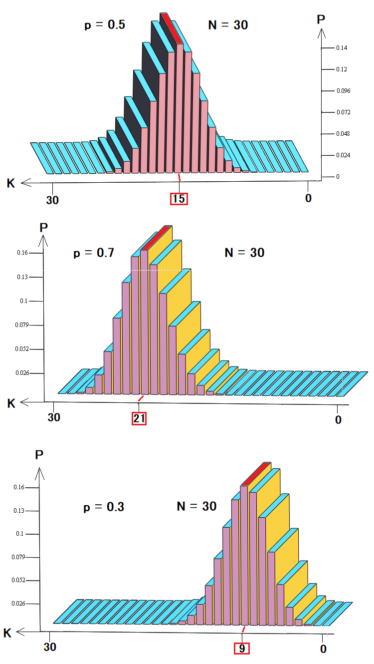
These three figures show:

1. Probability distribution in a random walk or trading
2. Probability distribution for profitable trading or an uptrend
3. Probability distribution for losing trading or downtrend

As can be seen from the diagrams, depending on the probability of a step up, the probabilities of certain combinations change and the most probable case shifts to the left or to the rights, like all other probabilities. This backtest or pricing representation is the simplest and preferred model for analysis. Such a model is quite sufficient for describing pricing; however, it is not enough to describe trading. Actually, the balance curve can contain various trades, which differ in terms of duration and profit/loss. Depending on which trading metrics are more important, we can set any desired number of states, not just two.

Multiple states

Now, let's consider the following example. Suppose we are still interested in the profit or loss value of a trade. Now, we know that the profit or loss state can take three strictly defined values, and we know the probabilities of each of the values. If this is the case, then we can say that we have a three-state system. Is it possible to describe all possible event developments like a two-state system? Actually, it is possible. I'm going to slightly improve the Bernoulli scheme so that it can work with a system with any number of states.

According to Bernoulli logic, we need to define state counters:

• i[0] – the number of outcomes with the first state in a chain of independent experiments
• i[1] is the number of outcomes with the second state in a chain of independent experiments
• . . .
• i[N] is the number of outcomes with the N – state
• N is the number of system states
• s is the state number

If we determine the number of occurrences of a certain state one by one, then the available number for the next state will be:

• s[i]  = N - Summ(0… k … i - 1) [ s[k] ]

It can be simplified. If we have chosen the number of outcomes of the previous state, then the number of outcomes for the next state remains exactly the same as the number of states that were selected for the previous state. Just like in the Bernoulli scheme, there are chains of probabilities that are inconsistent and have the same probability. The number of chains with the same number of all states is then calculated as follows:

• A[h](N,i[0]  ,i[1] ,… i[n]) = C(N , i[0]) * C(N-i[0] , i[1]) *…. C(N-Summ(0…k…n-1)[ i[k] ] , i[n])
• C are combinations
• h is a unique set of steps

Obviously, the probabilities of such sets can be calculated as in the Bernoulli scheme. Multiply the probability of one set by their number:

• P[k] = A[h](N,i[0]  ,i[1] ,… i[n]) * Pow(p[0], i[0]) * Pow(p[1], i[1]) … * Pow(1- Summ(0…j…N-1)[ p[j] ] , i[1])
• p[j] is the probability of a certain state

For clarity, I have created three-dimensional graphs, as in the previous example for two states. Again, we have 30 steps, but here we use three states instead of two:

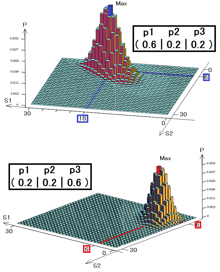
The volume of such a diagram will be exactly equal to one, since each bar symbolizes an incompatible event, and all these incompatible events just form a complete group. The diagrams show two different strategies with different probability vectors. These probabilities symbolize the chance of occurrence of one of the three states.

• S1 is the number of first state occurrences
• S2 is the number of second state occurrences
• S3 = 30 – S1 – S2 – the number of third state occurrences

If our system had a fourth state, then it could be presented only in a four-dimensional way. For five states we would need a five-dimensional diagram, and so on. For the human eye, only 3 dimensions are available, so more complex systems cannot be represented graphically. Nevertheless, multidimensional functions are also functional, just like the others.

Software implementation of multiple states

Two-state cases can be represented by a one-dimensional array. What about multiple states? We may think of a multidimensional array. But, as far as I know, all programming languages use at most two-dimensional arrays. Perhaps, some offer the possibility to create three or more-dimensional array, but this is not a convenient option. A better option is to use collections or tuples:

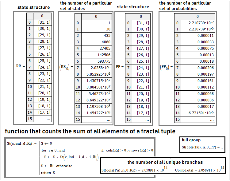
This is the situation with “30” steps. The first and third columns reflect the internal structure of the tuple. This is just an array within an array. Where it is written for example “[31,1]”, this means that this matrix element is also a matrix with “31” rows and one column. Bernoulli formula and the entire Bernoulli scheme are just a particular case of this more general scheme. If two states are required, the tuples will turn into one-dimensional arrays, in which case we will get simple combinations which play the key role in the Bernoulli formula.

If we look at what is inside these arrays, we will get columns “2” and “4”. The second column is the number of equivalent branches of specific unique sets of states, and the fourth is the total probability of such branches, because their probabilities are equal.

A truly clear criterion for validating the calculation of such tuples is to check the complete group of events and the total number of all unique branches. To do this, we can create a general function that will sum up all the elements of their complex tuples, no matter how complex their internal structure is. An example is shown in the screenshot above. Such a function must be recurrent; it should call itself inside — in this case it will be a universal function for any number of states and number of steps. As for the number of unique branches, the true value is calculated as follows:

• Pow(N,n)

In other words, the number of system states must be raised to the power of the number of steps - this way we will get all possible combinations of unique chains consisting of our states. In th figure, this number is shown as the “CombTotal” variable. The resulting sum will be compared to this variable.

In order to count the tuples, we should use similar functions with the same recurrent structure:

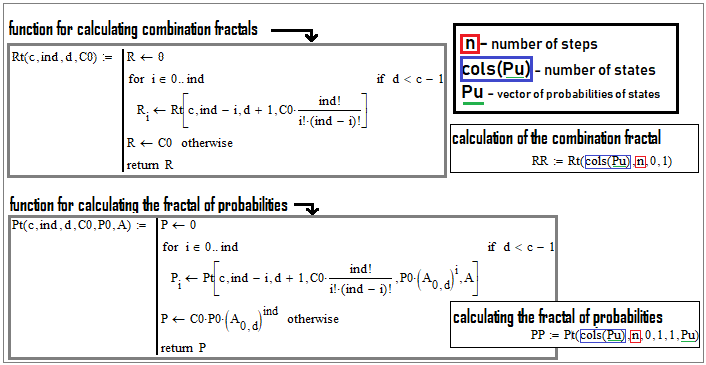
As you can see, they are very similar. There are just a couple of differences. At each level, we must additionally multiply the result by the number of combinations on the remaining free steps. When calculating the probabilities, the result must be additionally multiplied by the probability of the state currently under examination. Also, do not forget to multiply by the already accumulated probability of the chain. One by one accumulate all states until there are no free cells left, while the cells are the number of steps.

We can also consider an example of extracting states from the data that we know. For example, we have trading statistics, in which the following information is stored for each order: lifetime, trading volume, loss or profit, etc. Since the sample is finite, the number of states is also finite. For example, we can determine how many profit options there are in the sample. Each unique profit value can be considered a unique state. Count the number of occurrences of all such profits throughout the sample, divide by the total number of all deal and get the probability of a particular state. Repeat this for all states. If we then sum up all these probabilities, we get one. In this case everything is done correctly. In a similar way, we can classify trades by order lifetime. In other words, a state can be any unique characteristic of an event. In this case, a trade is considered an event, while the trade parameters are the characteristics of a particular event. In our case, the state examples can be as follow:

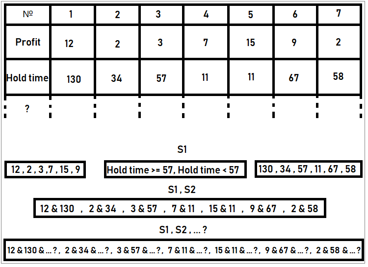
The figure shows an example of compiling sets of states. According to the rules, states should form a complete group of events, i.e. there should not be joint states there. The probability of these events can be calculated by dividing the number of orders in the table with specific states by the number of all orders (which is 7 in our case). This was the example of orders; however, we can work with any other states.

Conclusion

In this article, I tried to demonstrate how to evaluate data samples, how to make new ones from such samples by classifying the data and combining them into sets of states, the probabilities of which can be calculated. What to do with this data is up to you. I think the best use is to create multiple samples and to evaluate them — this is also called sample clustering. Sample clustering can serve as a good filter to enhance trading performance of existing systems. It can also be used to obtain profit from a seemingly unprofitable strategy — simply cluster the data and find the desired profitable samples. And most importantly, such mechanisms can be used as data processing stages in scalable trading systems. We will apply these mechanisms in practice later, when we move on to assembling a self-adapting trading system. For now, this is just another brick.

References

• Combinatorics and probability theory for trading (Part I): The basics
  
• Combinatorics and probability theory for trading (Part II): Universal fractal
  
• Combinatorics and probability theory for trading (Part III): The first mathematical model