用 MQL5 表示统计概率分布

MetaTrader 5 — 示例 | 2 一月 2014, 06:30

2 351

Denis Kirichenko

整个概率论以不可欲性 (undesirability) 哲学体系为基础。
(Leonid Sukhorukov)

简介

按活动的性质，交易者经常不得不将这些类别作为概率和随机性来对待。随机性的对立面是“规律性”概念。不同寻常的，借助普遍哲学规律，随机性作为一条规律转变为规律性。此时我们不讨论相反的过程。基本而言，随机性-规律性相关性是一种关键关系，因为，如果放在市场环境中考虑，它直接影响了交易者获得的盈利金额。

在本文中，我将列出基础理论工具，这些工具将在以后帮助我们发现某些市场规律。

1. 分布、本质、类型

那么，为了描述某些随机变量，我将需要一个一维统计概率分布。它将按某个规律描述随机变量样本，也就是说任何分布规律的应用都需要一组随机变量。

为什么分析[理论]分布？它们让依据变量属性值识别频率变化图形变得简单。此外，还可以获得所需分布的一些统计参数。

对于概率分布的类型，在专业文献中依据随机变量集合的类型将分布系列分为连续分布和离散分布是一个惯例。然而，还有其他分类，例如按分布曲线 f(x) 相对于曲线 x=x0 的对称性、位置参数、模式数量、随机变量区间等标准。

有几种方式来定义分布规律。我们应指出其中最流行的方式：

2. 理论概率分布

现在，让我们尝试在 MQL5 环境中创建描述统计分布的类。此外，我也要补充，专业文献提供了很多用 C++ 编写的代码示例，可以将这些示例成功应用到 MQL5 代码的编写。因此，我没有进行不必要的重复劳动，并且在某些情形中还使用了 C++ 代码最佳实践。

我面临的最大挑战是在 MQL5 中缺少多个继承支持。这是我为什么不尽量使用复杂的类的层次结构的原因。名为《Numerical Recipes:The Art of Scientific Computing》（数值算法：科学计算的艺术）一书 [2] 已经成为我的 C++ 代码的最佳来源，我从中借用了大多数函数。很多情况下必须依据 MQL5 的需要重新定义它们。

2.1.1 正态分布

按照传统，我们从正态分布开始。

正态分布也称为高斯分布，是概率密度函数给出的概率分布：

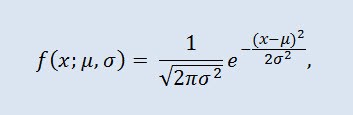
其中参数 μ 是随机变量的平均值（期望值），表示分布密度曲线的最大坐标，σ² 是方差。

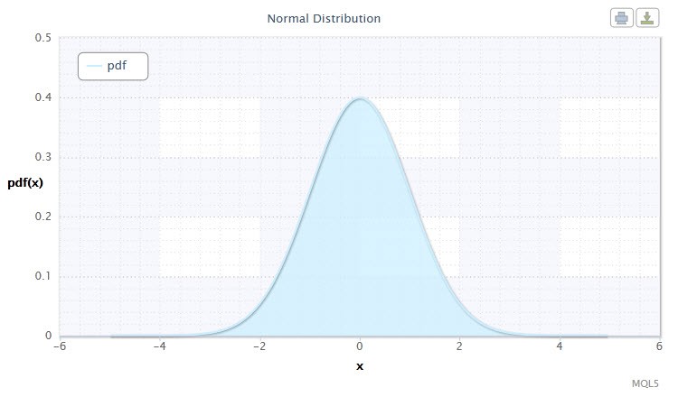
图 1. 正态分布密度 Nor(0,1)

其符号采用以下格式：X ~ Nor(μ, σ²)，其中：

X 是从正态分布 Nor 选择的随机变量；
μ 是平均值参数 (-∞ ≤ μ ≤ +∞)；
σ 是方差参数 (0<σ)。

随机变量 X 的有效范围： -∞ ≤ X ≤ +∞。

本文使用的公式可能与在其他资料中提供的公式有所不同。此类不同有时在数学上并不是至关紧要的。在某些情形中，它取决于参数表示的差异。

正态分布在统计中扮演了一个重要的角色，因为它反映了每一个都不具备主导力量的大量随机原因相互作用而造成的规律性。尽管正态分布在金融市场中很罕见，但是将它与经验分布进行比较以确定它们的异常程度和性质仍然非常重要。

让我们将用于正态分布的 CNormaldist 类定义为：

//+------------------------------------------------------------------+
//|                Normal Distribution class definition              |
//+------------------------------------------------------------------+
class CNormaldist : CErf // Erf class inheritance
  {
public:
   double            mu, //mean parameter (μ)
   sig;                 //variance parameter (σ)
   //+------------------------------------------------------------------+
   //| CNormaldist class constructor                                    |
   //+------------------------------------------------------------------+
   void  CNormaldist()
     {
      mu=0.0;sig=1.0; //default parameters μ and σ
      if(sig<=0.) Alert("bad sig in Normal Distribution!");
     }
   //+------------------------------------------------------------------+
   //| Probability density function (pdf)                               |
   //+------------------------------------------------------------------+
   double pdf(double x)
     {
      return(0.398942280401432678/sig)*exp(-0.5*pow((x-mu)/sig,2));
     }
   //+------------------------------------------------------------------+
   //| Cumulative distribution function (cdf)                           |
   //+------------------------------------------------------------------+
   double cdf(double x)
     {
      return 0.5*erfc(-0.707106781186547524*(x-mu)/sig);
     }
   //+------------------------------------------------------------------+
   //| Inverse cumulative distribution function (invcdf)                |
   //| quantile function                                                |
   //+------------------------------------------------------------------+
   double invcdf(double p)
     {
      if(!(p>0. && p<1.))
         Alert("bad p in Normal Distribution!");
      return -1.41421356237309505*sig*inverfc(2.*p)+mu;
     }
   //+------------------------------------------------------------------+
   //| Reliability (survival) function (sf)                             |
   //+------------------------------------------------------------------+
   double sf(double x)
     {
      return 1-cdf(x);
     }
  };

//+------------------------------------------------------------------+

您会注意到，CNormaldist 类派生于 СErf 基类，该类又定义误差函数类。在某些 CNormaldist 类方法的计算中需要它。СErf 类和辅助函数 erfcc 看起来或多或少如下所示：

//+------------------------------------------------------------------+
//|                Error Function class definition                   |
//+------------------------------------------------------------------+
class CErf
  {
public:
   int               ncof;    // coefficient array size
   double            cof[28]; // Chebyshev coefficient array
   //+------------------------------------------------------------------+
   //| CErf class constructor                                           |
   //+------------------------------------------------------------------+
   void CErf()
     {
      int Ncof=28;
      double Cof[28]=//Chebyshev coefficients
        {
         -1.3026537197817094,6.4196979235649026e-1,
         1.9476473204185836e-2,-9.561514786808631e-3,-9.46595344482036e-4,
         3.66839497852761e-4,4.2523324806907e-5,-2.0278578112534e-5,
         -1.624290004647e-6,1.303655835580e-6,1.5626441722e-8,-8.5238095915e-8,
         6.529054439e-9,5.059343495e-9,-9.91364156e-10,-2.27365122e-10,
         9.6467911e-11, 2.394038e-12,-6.886027e-12,8.94487e-13, 3.13092e-13,
         -1.12708e-13,3.81e-16,7.106e-15,-1.523e-15,-9.4e-17,1.21e-16,-2.8e-17
        };
      setCErf(Ncof,Cof);
     };
   //+------------------------------------------------------------------+
   //| Set-method for ncof                                              |
   //+------------------------------------------------------------------+
   void setCErf(int Ncof,double &Cof[])
     {
      ncof=Ncof;
      ArrayCopy(cof,Cof);
     };
   //+------------------------------------------------------------------+
   //| CErf class destructor                                            |
   //+------------------------------------------------------------------+
   void ~CErf(){};
   //+------------------------------------------------------------------+
   //| Error function                                                   |
   //+------------------------------------------------------------------+
   double erf(double x)
     {
      if(x>=0.0) return 1.0-erfccheb(x);
      else return erfccheb(-x)-1.0;
     }
   //+------------------------------------------------------------------+
   //| Complementary error function                                     |
   //+------------------------------------------------------------------+
   double erfc(double x)
     {
      if(x>=0.0) return erfccheb(x);
      else return 2.0-erfccheb(-x);
     }
   //+------------------------------------------------------------------+
   //| Chebyshev approximations for the error function                  |
   //+------------------------------------------------------------------+
   double erfccheb(double z)
     {
      int j;
      double t,ty,tmp,d=0.0,dd=0.0;
      if(z<0.) Alert("erfccheb requires nonnegative argument!");
      t=2.0/(2.0+z);
      ty=4.0*t-2.0;
      for(j=ncof-1;j>0;j--)
        {
         tmp=d;
         d=ty*d-dd+cof[j];
         dd=tmp;
        }
      return t*exp(-z*z+0.5*(cof[0]+ty*d)-dd);
     }
   //+------------------------------------------------------------------+
   //| Inverse complementary error function                             |
   //+------------------------------------------------------------------+
   double inverfc(double p)
     {
      double x,err,t,pp;
      if(p >= 2.0) return -100.0;
      if(p <= 0.0) return 100.0;
      pp=(p<1.0)? p : 2.0-p;
      t = sqrt(-2.*log(pp/2.0));
      x = -0.70711*((2.30753+t*0.27061)/(1.0+t*(0.99229+t*0.04481)) - t);
      for(int j=0;j<2;j++)
        {
         err=erfc(x)-pp;
         x+=err/(M_2_SQRTPI*exp(-pow(x,2))-x*err);
        }
      return(p<1.0? x : -x);
     }
   //+------------------------------------------------------------------+
   //| Inverse error function                                           |
   //+------------------------------------------------------------------+
   double inverf(double p)
     {return inverfc(1.0-p);}
  };
//+------------------------------------------------------------------+
double erfcc(const double x)
/* 
 complementary error function erfc(x) with
 a relative error of 1.2 * 10^(-7)               
*/
  {
   double t,z=fabs(x),ans;
   t=2./(2.0+z);
   ans=t*exp(-z*z-1.26551223+t*(1.00002368+t*(0.37409196+t*(0.09678418+
             t*(-0.18628806+t*(0.27886807+t*(-1.13520398+t*(1.48851587+
             t*(-0.82215223+t*0.17087277)))))))));
   return(x>=0.0 ? ans : 2.0-ans);
  }
//+------------------------------------------------------------------+

2.1.2 对数正态分布

现在，让我们看一看对数正态分布。

在概率论中，对数正态分布是一个两参数的绝对连续分布。如果随机变量是对数正态分布，则其对数为正态分布。

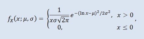
其中 μ 是位置参数 (0<μ )，σ 是比例参数 (0<σ)。

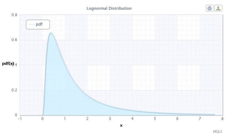
图 2. 对数正态分布密度 Logn(0,1)

其符号采用以下格式：X ~ Logn(μ, σ²)，其中：

X 是从对数正态分布 Logn 选择的随机变量；
μ 是位置参数 (0<μ )；
σ 是比例参数 (0<σ)。

随机变量 X 的有效范围：0 ≤ X ≤ +∞。

让我们创建 CLognormaldist 类，该类描述对数正态分布。它看起来如下所示：

//+------------------------------------------------------------------+
//|                Lognormal Distribution class definition           |
//+------------------------------------------------------------------+
class CLognormaldist : CErf // Erf class inheritance
  {
public:
   double            mu, //location parameter (μ)
   sig;                 //scale parameter (σ)
   //+------------------------------------------------------------------+
   //| CLognormaldist class constructor                                 |
   //+------------------------------------------------------------------+
   void  CLognormaldist()
     {
      mu=0.0;sig=1.0; //default parameters μ and σ
      if(sig<=0.) Alert("bad sig in Lognormal Distribution!");
     }
   //+------------------------------------------------------------------+
   //| Probability density function (pdf)                               |
   //+------------------------------------------------------------------+
   double pdf(double x)
     {
      if(x<0.) Alert("bad x in Lognormal Distribution!");
      if(x==0.) return 0.;
      return(0.398942280401432678/(sig*x))*exp(-0.5*pow((log(x)-mu)/sig,2));
     }
   //+------------------------------------------------------------------+
   //| Cumulative distribution function (cdf)                           |
   //+------------------------------------------------------------------+
   double cdf(double x)
     {
      if(x<0.) Alert("bad x in Lognormal Distribution!");
      if(x==0.) return 0.;
      return 0.5*erfc(-0.707106781186547524*(log(x)-mu)/sig);
     }
   //+------------------------------------------------------------------+
   //| Inverse cumulative distribution function (invcdf)(quantile)      |
   //+------------------------------------------------------------------+
   double invcdf(double p)
     {
      if(!(p>0. && p<1.))
         Alert("bad p in Lognormal Distribution!");
      return exp(-1.41421356237309505*sig*inverfc(2.*p)+mu);
     }
   //+------------------------------------------------------------------+
   //| Reliability (survival) function (sf)                             |
   //+------------------------------------------------------------------+
   double sf(double x)
     {
      return 1-cdf(x);
     }
  };
//+------------------------------------------------------------------+

如您所见，对数正态分布与正态分布并没有很大的不同。区别在于参数 x 被参数 log(x) 代替。

2.1.3 柯西分布

概率论中的柯西分布（在物理学中也称为洛伦兹分布或布赖特-维格纳分布）是一类绝对连续分布。服从柯西分布的随机变量是没有期望值和方差的变量的一个常见例子。密度采用以下形式：

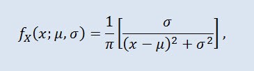
其中 μ 是位置参数 (-∞ ≤ μ ≤ +∞ )，σ 是比例参数 (0<σ)。

柯西分布的符号采用以下格式：X ~ Cau(μ, σ)，其中：

X 是从柯西分布 Cau 选择的随机变量；
μ 是位置参数 (-∞ ≤ μ ≤ +∞)；
σ 是比例参数 (0<σ)。

随机变量 X 的有效范围： -∞ ≤ X ≤ +∞。

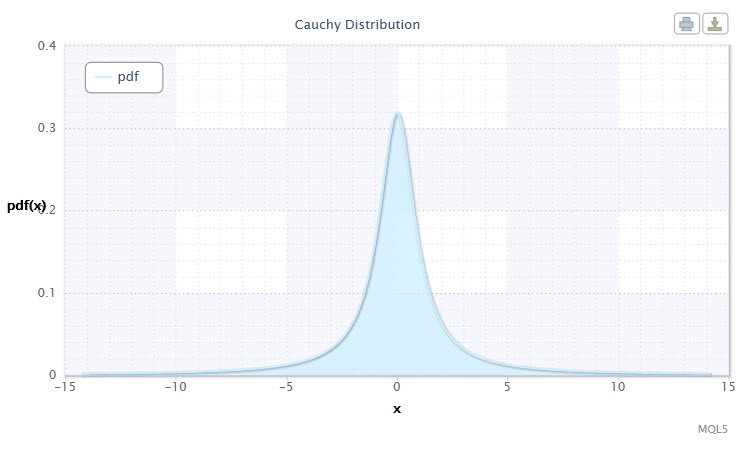
图 3. 柯西分布密度 Cau(0,1)

以 MQL5 格式，在 CCauchydist 类的帮助下创建，它看起来如下所示：

//+------------------------------------------------------------------+
//|                Cauchy Distribution class definition              |
//+------------------------------------------------------------------+
class CCauchydist //
  {
public:
   double            mu,//location parameter (μ)
   sig;                 //scale parameter (σ)
   //+------------------------------------------------------------------+
   //| CCauchydist class constructor                                    |
   //+------------------------------------------------------------------+
   void  CCauchydist() 
     {
      mu=0.0;sig=1.0; //default parameters μ and σ
      if(sig<=0.) Alert("bad sig in Cauchy Distribution!");
     }
   //+------------------------------------------------------------------+
   //| Probability density function (pdf)                               |
   //+------------------------------------------------------------------+
   double pdf(double x)
     {
      return 0.318309886183790671/(sig*(1.+pow((x-mu)/sig,2)));
     }
   //+------------------------------------------------------------------+
   //| Cumulative distribution function (cdf)                           |
   //+------------------------------------------------------------------+
   double cdf(double x)
     {
      return 0.5+0.318309886183790671*atan2(x-mu,sig); //todo      
     }
   //+------------------------------------------------------------------+
   //| Inverse cumulative distribution function (invcdf) (quantile func)|
   //+------------------------------------------------------------------+
   double invcdf(double p)
     {
      if(!(p>0. && p<1.))
         Alert("bad p in Cauchy Distribution!");
      return mu+sig*tan(M_PI*(p-0.5));
     }
   //+------------------------------------------------------------------+
   //| Reliability (survival) function (sf)                             |
   //+------------------------------------------------------------------+
   double sf(double x)
     {
      return 1-cdf(x);
     }
  };
//+------------------------------------------------------------------+

应在这里指出，采用了 atan2() 函数，它以弧度为单位返回反正切的主值：

double atan2(double y,double x)
/*
 Returns the principal value of the arc tangent of y/x,
 expressed in radians. To compute the value, the function 
 uses the sign of both arguments to determine the quadrant.
 y - double value representing an y-coordinate.
 x - double value representing an x-coordinate. 
*/
  {
   double a;
   if(fabs(x)>fabs(y))
      a=atan(y/x);
   else
     {
      a=atan(x/y); // pi/4 <= a <= pi/4
      if(a<0.)
         a=-1.*M_PI_2-a; //a is negative, so we're adding
      else
         a=M_PI_2-a;
     }
   if(x<0.)
     {
      if(y<0.)
         a=a-M_PI;
      else
         a=a+M_PI;
     }
   return a;
  }

2.1.4 双曲线正割分布

双曲线正割分布会让那些处理金融排名分析的人感兴趣。

在概率论和统计学中，双曲线正割分布是一种连续分布，其概率密度函数和特征函数与双曲线正割函数成正比。密度按以下公式给出：

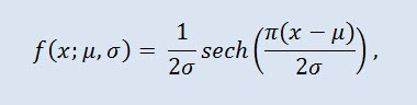
其中 μ 是位置参数 (-∞ ≤ μ ≤ +∞ )，σ 是比例参数 (0<σ)。

图 4. 双曲线正割分布密度 HS(0,1)

其符号采用以下格式：X ~ HS(μ, σ)，其中：

X 是随机变量；
μ 是位置参数 (-∞ ≤ μ ≤ +∞)；
σ 是比例参数 (0<σ)。

随机变量 X 的有效范围： -∞ ≤ X ≤ +∞。

让我们使用 CHypersecdist 类来描述它，如下所示：

//+------------------------------------------------------------------+
//|        Hyperbolic Secant Distribution class definition           |
//+------------------------------------------------------------------+
class CHypersecdist //
  {
public:
   double            mu,// location parameter (μ)
   sig;                 //scale parameter (σ)
   //+------------------------------------------------------------------+
   //| CHypersecdist class constructor                                 |
   //+------------------------------------------------------------------+
   void  CHypersecdist()
     {
      mu=0.0;sig=1.0; //default parameters μ and σ
      if(sig<=0.) Alert("bad sig in Hyperbolic Secant Distribution!");
     }
   //+------------------------------------------------------------------+
   //| Probability density function (pdf)                               |
   //+------------------------------------------------------------------+
   double pdf(double x)
     {
      return sech((M_PI*(x-mu))/(2*sig))/2*sig;
     }
   //+------------------------------------------------------------------+
   //| Cumulative distribution function (cdf)                           |
   //+------------------------------------------------------------------+
   double cdf(double x)
     {
      return 2/M_PI*atan(exp((M_PI*(x-mu)/(2*sig))));
     }
   //+------------------------------------------------------------------+
   //| Inverse cumulative distribution function (invcdf) (quantile func)|
   //+------------------------------------------------------------------+
   double invcdf(double p)
     {
      if(!(p>0. && p<1.))
         Alert("bad p in Hyperbolic Secant Distribution!");
      return(mu+(2.0*sig/M_PI*log(tan(M_PI/2.0*p))));
     }
   //+------------------------------------------------------------------+
   //| Reliability (survival) function (sf)                             |
   //+------------------------------------------------------------------+
   double sf(double x)
     {
      return 1-cdf(x);
     }
  };
//+------------------------------------------------------------------+

不难看出，此分布得名于双曲线正割函数，其概率密度函数与双曲线正割函数成正比。

双曲线正割函数 sech 如下所示：

//+------------------------------------------------------------------+
//|              Hyperbolic Secant Function                          |
//+------------------------------------------------------------------+
double sech(double x)
// Hyperbolic Secant Function
  {
   return 2/(pow(M_E,x)+pow(M_E,-x));
  }

2.1.5 学生 t 分布

学生 t 分布在统计学中是一种重要的分布。

在概率论中，学生 t 分布通常是一参数系列的绝对连续分布。然而，也可以视为分布密度函数产生的三参数分布：

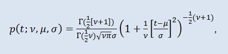
其中，Г 是殴拉的伽玛函数，ν 是形状参数 (ν>0)，μ 是位置参数 (-∞ ≤ μ ≤ +∞ )，σ 是比例参数 (0<σ)。

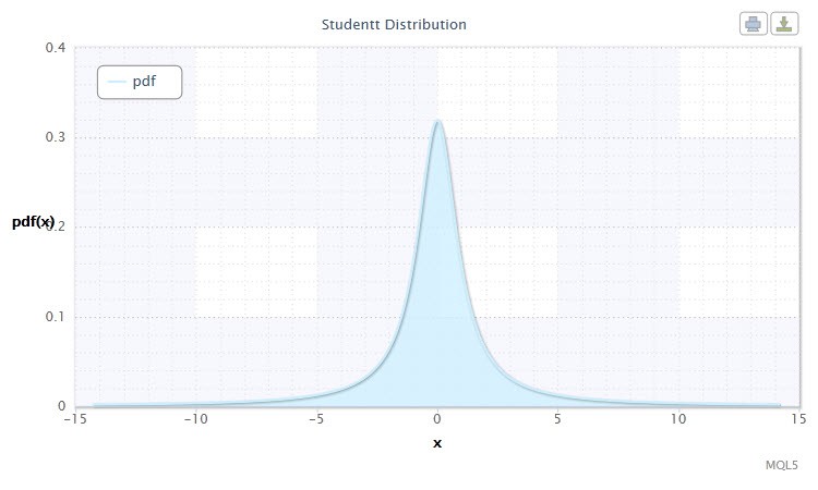
图 5. 学生 t 分布密度 Stt(1,0,1)

其符号采用以下格式：t ~ Stt(ν,μ,σ)，其中：

t 是从学生 t 分布 Stt 选择的随机变量；
ν 是形状参数 (ν>0)
μ 是位置参数 (-∞ ≤ μ ≤ +∞)；
σ 是比例参数 (0<σ)。

随机变量 X 的有效范围： -∞ ≤ X ≤ +∞。

通常，尤其是在假设测试中，使用 μ=0 和 σ=1 的标准 t 分布。因此，它转换为含有参数 v 的一参数分布。

在测试期望值假设、回归关系系数、同质性假设时，经常用此分布通过置信区间估计期望值，预测值和其他特征。

让我们通过 CStudenttdist 类描述此分布：

//+------------------------------------------------------------------+
//|                Student's t-distribution class definition         |
//+------------------------------------------------------------------+
class CStudenttdist : CBeta // CBeta class inheritance
  {
public:
   int               nu;     // shape parameter (ν)
   double            mu,     // location parameter (μ)
   sig,                     // scale parameter (σ)
   np,                      // 1/2*(ν+1)
   fac;                     // Г(1/2*(ν+1))-Г(1/2*ν)
   //+------------------------------------------------------------------+
   //| CStudenttdist class constructor                                  |
   //+------------------------------------------------------------------+
   void  CStudenttdist()
     {
      int Nu=1;double Mu=0.0,Sig=1.0; //default parameters ν, μ and σ
      setCStudenttdist(Nu,Mu,Sig);
     }
   void setCStudenttdist(int Nu,double Mu,double Sig)
     {
      nu=Nu;
      mu=Mu;
      sig=Sig;
      if(sig<=0. || nu<=0.) Alert("bad sig,nu in Student-t Distribution!");
      np=0.5*(nu+1.);
      fac=gammln(np)-gammln(0.5*nu);
     }
   //+------------------------------------------------------------------+
   //| Probability density function (pdf)                               |
   //+------------------------------------------------------------------+
   double pdf(double x)
     {
      return exp(-np*log(1.+pow((x-mu)/sig,2.)/nu)+fac)/(sqrt(M_PI*nu)*sig);
     }
   //+------------------------------------------------------------------+
   //| Cumulative distribution function (cdf)                           |
   //+------------------------------------------------------------------+
   double cdf(double t)
     {
      double p=0.5*betai(0.5*nu,0.5,nu/(nu+pow((t-mu)/sig,2)));
      if(t>=mu) return 1.-p;
      else return p;
     }
   //+------------------------------------------------------------------+
   //| Inverse cumulative distribution function (invcdf) (quantile func)|
   //+------------------------------------------------------------------+
   double invcdf(double p)
     {
      if(p<=0. || p>=1.) Alert("bad p in Student-t Distribution!");
      double x=invbetai(2.*fmin(p,1.-p),0.5*nu,0.5);
      x=sig*sqrt(nu*(1.-x)/x);
      return(p>=0.5? mu+x : mu-x);
     }
   //+------------------------------------------------------------------+
   //| Reliability (survival) function (sf)                             |
   //+------------------------------------------------------------------+
   double sf(double x)
     {
      return 1-cdf(x);
     }
   //+------------------------------------------------------------------+
   //| Two-tailed cumulative distribution function (aa) A(t|ν)          |
   //+------------------------------------------------------------------+
   double aa(double t)
     {
      if(t < 0.) Alert("bad t in Student-t Distribution!");
      return 1.-betai(0.5*nu,0.5,nu/(nu+pow(t,2.)));
     }
   //+------------------------------------------------------------------+
   //| Inverse two-tailed cumulative distribution function (invaa)      |
   //| p=A(t|ν)                                                         |
   //+------------------------------------------------------------------+
   double invaa(double p)
     {
      if(!(p>=0. && p<1.)) Alert("bad p in Student-t Distribution!");
      double x=invbetai(1.-p,0.5*nu,0.5);
      return sqrt(nu*(1.-x)/x);
     }
  };
//+------------------------------------------------------------------+

CStudenttdist 类的清单显示 CBeta 是基类，该类描述不完整的贝塔函数。

CBeta 类看起来如下所示：

//+------------------------------------------------------------------+
//|            Incomplete Beta Function class definition             |
//+------------------------------------------------------------------+
class CBeta : public CGauleg18
  {
private:
   int               Switch;                     //when to use the quadrature method
   double            Eps,Fpmin;
public:
   //+------------------------------------------------------------------+
   //| CBeta class constructor                                          |
   //+------------------------------------------------------------------+
   void CBeta()
     {
      int swi=3000;
      setCBeta(swi,EPS,FPMIN);
     };
   //+------------------------------------------------------------------+
   //| CBeta class set-method                                           |
   //+------------------------------------------------------------------+
   void setCBeta(int swi,double eps,double fpmin)
     {
      Switch=swi;
      Eps=eps;
      Fpmin=fpmin;
     };
   double            betai(const double a,const double b,const double x); //incomplete beta function Ix(a,b)
   double            betacf(const double a,const double b,const double x);//continued fraction for incomplete beta function
   double            betaiapprox(double a,double b,double x); //Incomplete beta by quadrature
   double            invbetai(double p,double a,double b);    //Inverse of incomplete beta function
  };

这个类也有一个基类 CGauleg18，该类为诸如高斯-勒让德求积分法等数值积分方法提供系数。

2.1.6 逻辑分布

我建议在我们的研究中接下来考虑逻辑分布。

在概率论和统计学中，逻辑分布是一种连续概率分布。其累积分布函数是逻辑函数。它在形态上类似于正态分类，但是有更重的尾巴。分布密度：

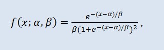
其中 α 是位置参数 (-∞ ≤ α ≤ +∞ )，β 是比例参数 (0<β)。

图 6. 逻辑分布密度Logi(0,1)

其符号采用以下格式：X ~ Logi(α,β)，其中：

X 是随机变量；
α 是位置参数 (-∞ ≤ α ≤ +∞ )；
β 是比例参数 (0<β)。

随机变量 X 的有效范围： -∞ ≤ X ≤ +∞。

CLogisticdist 类是上述分布的实施：

//+------------------------------------------------------------------+
//|                Logistic Distribution class definition            |
//+------------------------------------------------------------------+
class CLogisticdist
  {
public:
   double            alph,//location parameter (α)
   bet;                   //scale parameter (β)
   //+------------------------------------------------------------------+
   //| CLogisticdist class constructor                                  |
   //+------------------------------------------------------------------+
   void  CLogisticdist() 
     {
      alph=0.0;bet=1.0; //default parameters μ and σ
      if(bet<=0.) Alert("bad bet in Logistic Distribution!");
     }
   //+------------------------------------------------------------------+
   //| Probability density function (pdf)                               |
   //+------------------------------------------------------------------+
   double pdf(double x)
     {
      return exp(-(x-alph)/bet)/(bet*pow(1.+exp(-(x-alph)/bet),2));
     }
   //+------------------------------------------------------------------+
   //| Cumulative distribution function (cdf)                           |
   //+------------------------------------------------------------------+
   double cdf(double x)
     {
      double et=exp(-1.*fabs(1.81379936423421785*(x-alph)/bet));
      if(x>=alph) return 1./(1.+et);
      else return et/(1.+et);
     }
   //+------------------------------------------------------------------+
   //| Inverse cumulative distribution function (invcdf) (quantile func)|
   //+------------------------------------------------------------------+
   double invcdf(double p)
     {
      if(p<=0. || p>=1.) Alert("bad p in Logistic Distribution!");
      return alph+0.551328895421792049*bet*log(p/(1.-p));
     }
   //+------------------------------------------------------------------+
   //| Reliability (survival) function (sf)                             |
   //+------------------------------------------------------------------+
   double sf(double x)
     {
      return 1-cdf(x);
     }
  };
//+------------------------------------------------------------------+

2.1.7 指数分布

让我们再看一看随机变量的指数分布。

如果其密度符合以下公式，则随机变量 X 服从带有参数 λ > 0 的指数分布：

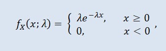
其中 λ 是比例参数 (λ>0)。

图 7. 指数分布密度 Exp(1)

其符号采用以下格式：X ~ Exp(λ)，其中：

X 是随机变量；
λ 是比例参数 (λ>0)。

随机变量 X 的有效范围：0 ≤ X ≤ +∞。

这个分布因为它描述在某些时间逐个发生的一系列事件而引人注目。因此，交易者可以使用这个分布来分析一系列的亏损交易和其他事件。

在 MQL5 代码中，通过 CExpondist 类描述该分布：

//+------------------------------------------------------------------+
//|                Exponential Distribution class definition         |
//+------------------------------------------------------------------+
class CExpondist
  {
public:
   double            lambda;   //scale parameter (λ)
   //+------------------------------------------------------------------+
   //| CExpondist class constructor                                     |
   //+------------------------------------------------------------------+
   void  CExpondist()
     {
      lambda=1.0;              //default parameter λ
      if(lambda<=0.) Alert("bad lambda in Exponential Distribution!");
     }
   //+------------------------------------------------------------------+
   //| Probability density function (pdf)                               |
   //+------------------------------------------------------------------+
   double pdf(double x)
     {
      if(x<0.) Alert("bad x in Exponential Distribution!");
      return lambda*exp(-lambda*x);
     }
   //+------------------------------------------------------------------+
   //| Cumulative distribution function (cdf)                           |
   //+------------------------------------------------------------------+
   double cdf(double x)
     {
      if(x < 0.) Alert("bad x in Exponential Distribution!");
      return 1.-exp(-lambda*x);
     }
   //+------------------------------------------------------------------+
   //| Inverse cumulative distribution function (invcdf) (quantile func)|
   //+------------------------------------------------------------------+
   double invcdf(double p)
     {
      if(p<0. || p>=1.) Alert("bad p in Exponential Distribution!");
      return -log(1.-p)/lambda;
     }
   //+------------------------------------------------------------------+
   //| Reliability (survival) function (sf)                             |
   //+------------------------------------------------------------------+
   double sf(double x)
     {
      return 1-cdf(x);
     }
  };
//+------------------------------------------------------------------+

2.1.8 伽玛分布

我选择伽玛分布作为随机变量连续分布的下一类型。

在概率论中，伽玛分布是一个两参数系列的绝对连续概率分布。如果参数 α 是一个整数，则此类伽玛分布也称为埃尔朗分布。密度采用以下形式：

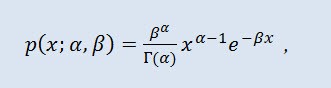
其中，Г 是殴拉的伽玛函数，α 是形状参数 (0<α)，β 是比例参数 (0<β)。

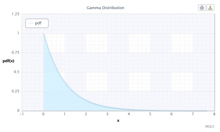
图 8. 伽玛分布密度 Gam(1,1)。

其符号采用以下格式：X ~ Gam(α,β)，其中：

X 是随机变量；
α 是形状参数 (0<α)；
β 是比例参数 (0<β)。

随机变量 X 的有效范围：0 ≤ X ≤ +∞。

在 CGammadist 类中定义的形式看起来如下所示：

//+------------------------------------------------------------------+
//|                Gamma Distribution class definition               |
//+------------------------------------------------------------------+
class CGammadist : CGamma // CGamma class inheritance
  {
public:
   double            alph,//continuous shape parameter (α>0)
   bet,                   //continuous scale parameter  (β>0)
   fac;                   //factor
   //+------------------------------------------------------------------+
   //| CGammaldist class constructor                                    |
   //+------------------------------------------------------------------+
   void  CGammadist()
     {
      setCGammadist();
     }
   void setCGammadist(double Alph=1.0,double Bet=1.0)//default parameters α and β
     {
      alph=Alph; bet=Bet;
      if(alph<=0. || bet<=0.) Alert("bad alph,bet in Gamma Distribution!");
      fac=alph*log(bet)-gammln(alph);
     }
   //+------------------------------------------------------------------+
   //| Probability density function (pdf)                               |
   //+------------------------------------------------------------------+
   double pdf(double x)
     {
      if(x<=0.) Alert("bad x in Gamma Distribution!");
      return exp(-bet*x+(alph-1.)*log(x)+fac);
     }
   //+------------------------------------------------------------------+
   //| Cumulative distribution function (cdf)                           |
   //+------------------------------------------------------------------+
   double cdf(double x)
     {
      if(x<0.) Alert("bad x in Gamma Distribution!");
      return gammp(alph,bet*x);
     }
   //+------------------------------------------------------------------+
   //| Inverse cumulative distribution function (invcdf) (quantile func)|
   //+------------------------------------------------------------------+
   double invcdf(double p)
     {
      if(p<0. || p>=1.) Alert("bad p in Gamma Distribution!");
      return invgammp(p,alph)/bet;
     }
   //+------------------------------------------------------------------+
   //| Reliability (survival) function (sf)                             |
   //+------------------------------------------------------------------+
   double sf(double x)
     {
      return 1-cdf(x);
     }
  };
//+------------------------------------------------------------------+

伽玛分布类派生于 CGamma 类，该类描述不完整的伽玛函数。

CGamma 类的定义如下所示：

//+------------------------------------------------------------------+
//|            Incomplete Gamma Function class definition            |
//+------------------------------------------------------------------+
class CGamma : public CGauleg18
  {
private:
   int               ASWITCH;
   double            Eps,
   Fpmin,
   gln;
public:
   //+------------------------------------------------------------------+
   //| CGamma class constructor                                         |
   //+------------------------------------------------------------------+
   void CGamma()
     {
      int aswi=100;
      setCGamma(aswi,EPS,FPMIN);
     };
   void setCGamma(int aswi,double eps,double fpmin) //CGamma set-method
     {
      ASWITCH=aswi;
      Eps=eps;
      Fpmin=fpmin;
     };
   double            gammp(const double a,const double x); //incomplete gamma function
   double            gammq(const double a,const double x); //incomplete gamma function Q(a,x)
   void              gser(double &gamser,double a,double x,double &gln); //incomplete gamma function P(a,x)
   double            gcf(const double a,const double x); //incomplete gamma function Q(a,x)
   double            gammpapprox(double a,double x,int psig); //incomplete gamma by quadrature
   double            invgammp(double p,double a); //inverse of incomplete gamma function
  };
//+------------------------------------------------------------------+

CGamma 类和 CBeta 类都有 CGauleg18 类作为基类。

2.1.9 贝塔分布

现在，让我们查看贝塔分布。

在概率论和统计学中，贝塔分布是一个两参数系列的绝对连续概率分布。它用于描述其值在有限区间内定义的随机变量。密度的定义如下：

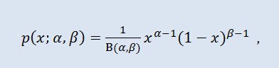
其中 B 是贝塔函数，α 是第一个形状参数 (0<α)，β 是第二个形状参数 (0<β)。

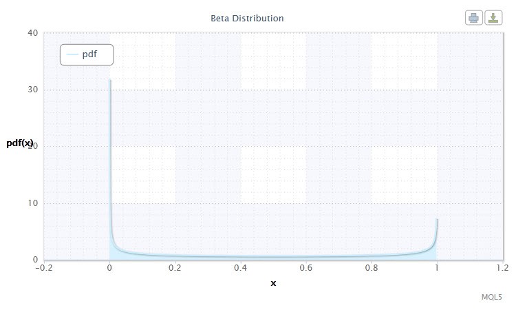
图 9. 贝塔分布密度 Beta(0.5,0.5)

其符号采用以下格式：X ~ Beta(α,β)，其中：

X 是随机变量；
α 是第一个形状参数 (0<α)；
β 是第二个形状参数 (0<β)。

随机变量 X 的有效范围：0 ≤ X ≤ 1。

CBetadist 类通过以下方式描述这个分布：

//+------------------------------------------------------------------+
//|                Beta Distribution class definition                |
//+------------------------------------------------------------------+
class CBetadist : CBeta // CBeta class inheritance
  {
public:
   double            alph,//continuous shape parameter (α>0)
   bet,                   //continuous shape parameter (β>0)
   fac;                   //factor
   //+------------------------------------------------------------------+
   //| CBetadist class constructor                                      |
   //+------------------------------------------------------------------+
   void  CBetadist()
     {
      setCBetadist();
     }
   void setCBetadist(double Alph=0.5,double Bet=0.5)//default parameters α and β
     {
      alph=Alph; bet=Bet;
      if(alph<=0. || bet<=0.) Alert("bad alph,bet in Beta Distribution!");
      fac=gammln(alph+bet)-gammln(alph)-gammln(bet);
     }
   //+------------------------------------------------------------------+
   //| Probability density function (pdf)                               |
   //+------------------------------------------------------------------+
   double pdf(double x)
     {
      if(x<=0. || x>=1.) Alert("bad x in Beta Distribution!");
      return exp((alph-1.)*log(x)+(bet-1.)*log(1.-x)+fac);
     }
   //+------------------------------------------------------------------+
   //| Cumulative distribution function (cdf)                           |
   //+------------------------------------------------------------------+
   double cdf(double x)
     {
      if(x<0. || x>1.) Alert("bad x in Beta Distribution");
      return betai(alph,bet,x);
     }
   //+------------------------------------------------------------------+
   //| Inverse cumulative distribution function (invcdf) (quantile func)|
   //+------------------------------------------------------------------+
   double invcdf(double p)
     {
      if(p<0. || p>1.) Alert("bad p in Beta Distribution!");
      return invbetai(p,alph,bet);
     }
   //+------------------------------------------------------------------+
   //| Reliability (survival) function (sf)                             |
   //+------------------------------------------------------------------+
   double sf(double x)
     {
      return 1-cdf(x);
     }
  };
//+------------------------------------------------------------------+

2.1.10 拉普拉斯分布

另一个引人注目的连续分布为拉普拉斯分布（双指数分布）。

在概率论中，拉普拉斯分布（双指数分布）是一种随机变量连续分布，其中概率密度为：

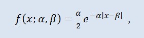
其中 α 是位置参数 (-∞ ≤ α ≤ +∞ )，β 是比例参数 (0<β)。

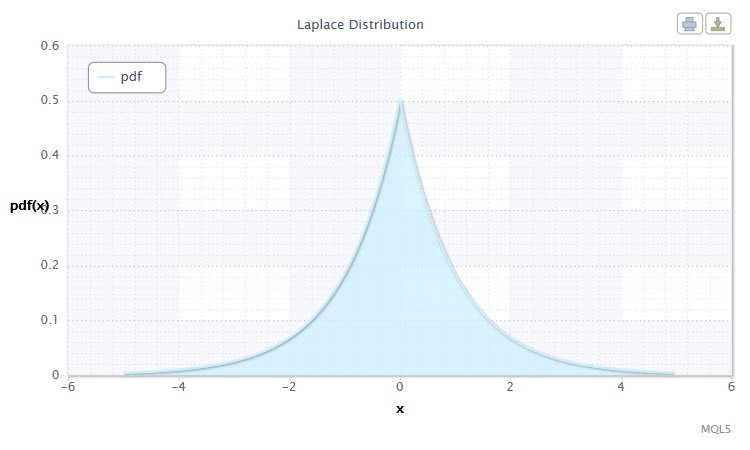
图 10. 拉普拉斯分布密度 Lap(0,1)

其符号采用以下格式：X ~ Lap(α,β)，其中：

X 是随机变量；
α 是位置参数 (-∞ ≤ α ≤ +∞ )；
β 是比例参数 (0<β)。

随机变量 X 的有效范围： -∞ ≤ X ≤ +∞。

用于此分布的 CLaplacedist 类定义如下：

//+------------------------------------------------------------------+
//|                 Laplace Distribution class definition            |
//+------------------------------------------------------------------+
class CLaplacedist
  {
public:
   double            alph;   //location parameter (α)
   double            bet;    //scale parameter (β)
   //+------------------------------------------------------------------+
   //| CLaplacedist class constructor                                   |
   //+------------------------------------------------------------------+
   void  CLaplacedist()
     {
      alph=.0;               //default parameter α
      bet=1.;                //default parameter β
      if(bet<=0.) Alert("bad bet in Laplace Distribution!");
     }
   //+------------------------------------------------------------------+
   //| Probability density function (pdf)                               |
   //+------------------------------------------------------------------+
   double pdf(double x)
     {
      return exp(-fabs((x-alph)/bet))/2*bet;
     }
   //+------------------------------------------------------------------+
   //| Cumulative distribution function (cdf)                           |
   //+------------------------------------------------------------------+
   double cdf(double x)
     {
      double temp;
      if(x<0)
         temp=0.5*exp(-fabs((x-alph)/bet));
      else
         temp=1.-0.5*exp(-fabs((x-alph)/bet));
      return temp;
     }
   //+------------------------------------------------------------------+
   //| Inverse cumulative distribution function (invcdf) (quantile func)|
   //+------------------------------------------------------------------+
   double invcdf(double p)
     {
      double temp;
      if(p<0. || p>=1.) Alert("bad p in Laplace Distribution!");
      if(p<0.5)
         temp=bet*log(2*p)+alph;
      else
         temp=-1.*(bet*log(2*(1.-p))+alph);
      return temp;
     }
   //+------------------------------------------------------------------+
   //| Reliability (survival) function (sf)                             |
   //+------------------------------------------------------------------+
   double sf(double x)
     {
      return 1-cdf(x);
     }
  };
//+------------------------------------------------------------------+

目前为止，我们使用 MQL5 代码为十个连续分布创建了 10 个类。此外，还创建了一些可以说是补充性的类，因为在具体的函数和方法中有这种需要（例如 CBeta 和 CGamma）。

现在，让我们继续介绍离散分布并为这种分布类型创建几个类。

2.2.1 二项分布

让我们从二项分布开始。

在概率论中，二项分布是在一系列的独立随机试验中成功次数的分布，其中每次试验的成功概率是相等的。概率密度按以下公式给出：

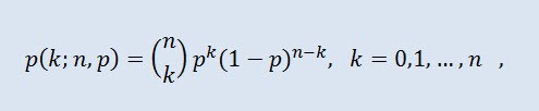
其中 (n k) 是二项式系数，n 是试验的次数 (0 ≤ n)，p 是成功概率 (0 ≤ p ≤1)。

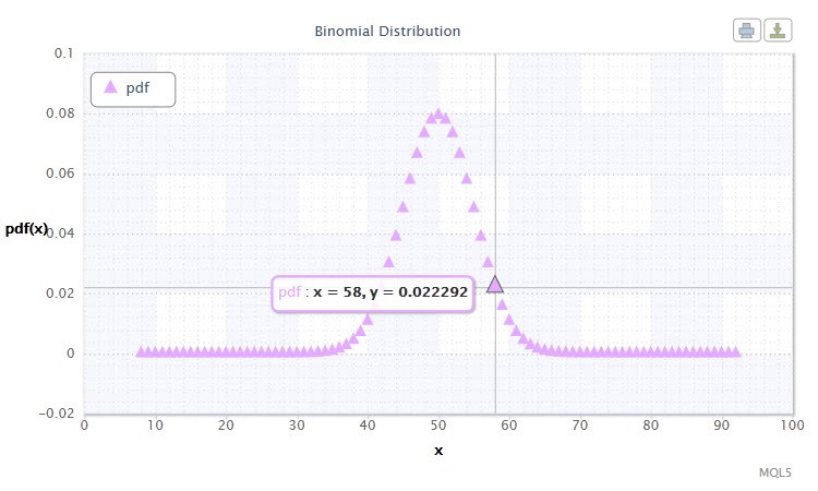
图 11. 二项分布密度 Bin(100,0.5)。

其符号采用以下格式：k ~ Bin(n,p)，其中：

k 是随机变量；
n 是试验次数 (0 ≤ n);
p 是成功概率 (0 ≤ p ≤1)。

随机变量 X 的有效范围：0 或 1。

随机变量 X 的可能取值范围对您有什么启示？事实上，这个分布可帮助我们分析交易系统中盈利 (1) 和亏损 (0) 交易的总数。

让我们创建如下所示的 СBinomialdist 类：

//+------------------------------------------------------------------+
//|               Binomial Distribution class definition             |
//+------------------------------------------------------------------+
class CBinomialdist : CBeta // CBeta class inheritance
  {
public:
   int               n;      //number of trials
   double            pe,     //success probability
   fac;                      //factor
   //+------------------------------------------------------------------+
   //| CBinomialdist class constructor                                  |
   //+------------------------------------------------------------------+
   void              CBinomialdist()
     {
      setCBinomialdist();
     }
   void setCBinomialdist(int N=100,double Pe=0.5)//default parameters n and pe
     {
      n=N; pe=Pe;
      if(n<=0 || pe<=0. || pe>=1.) Alert("bad args in Binomial Distribution!");
      fac=gammln(n+1.);
     }
   //+------------------------------------------------------------------+
   //| Probability density function (pdf)                               |
   //+------------------------------------------------------------------+
   double pdf(int k)
     {
      if(k<0) Alert("bad k in Binomial Distribution!");
      if(k>n) return 0.;
      return exp(k*log(pe)+(n-k)*log(1.-pe)+fac-gammln(k+1.)-gammln(n-k+1.));
     }
   //+------------------------------------------------------------------+
   //| Cumulative distribution function (cdf)                           |
   //+------------------------------------------------------------------+
   double cdf(int k)
     {
      if(k<0) Alert("bad k in Binomial Distribution!");
      if(k==0) return 0.;
      if(k>n) return 1.;
      return 1.-betai((double)k,n-k+1.,pe);
     }
   //+------------------------------------------------------------------+
   //| Inverse cumulative distribution function (invcdf) (quantile func)|
   //+------------------------------------------------------------------+
   int invcdf(double p)
     {
      int k,kl,ku,inc=1;
      if(p<=0. || p>=1.) Alert("bad p in Binomial Distribution!");
      k=fmax(0,fmin(n,(int)(n*pe)));
      if(p<cdf(k))
        {
         do
           {
            k=fmax(k-inc,0);
            inc*=2;
           }
         while(p<cdf(k));
         kl=k; ku=k+inc/2;
           } else {
         do
           {
            k=fmin(k+inc,n+1);
            inc*=2;
           }
         while(p>cdf(k));
         ku=k; kl=k-inc/2;
        }
      while(ku-kl>1)
        {
         k=(kl+ku)/2;
         if(p<cdf(k)) ku=k;
         else kl=k;
        }
      return kl;
     }
   //+------------------------------------------------------------------+
   //| Reliability (survival) function (sf)                             |
   //+------------------------------------------------------------------+
   double sf(int k)
     {
      return 1.-cdf(k);
     }
  };
//+------------------------------------------------------------------+

2.2.2 泊松分布

要查看的下一个分布是泊松分布。

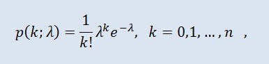
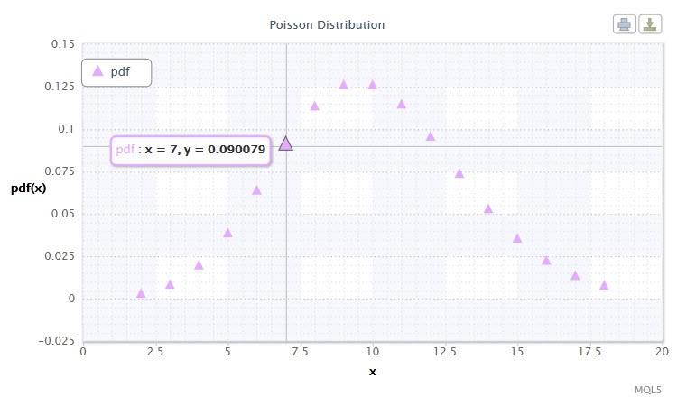
泊松分布对用在固定时间内发生的事件的次数表示的随机变量建模，前提是这些事件以固定的平均密度相互独立地发生。密度采用以下形式：

其中 k! 是阶乘，λ 是位置参数 (0 < λ)。

图 12. 泊松分布密度 Pois(10)。

其符号采用以下格式：k ~ Pois(λ)，其中：

k 是随机变量；
λ 是位置参数 (0 < λ)。

随机变量 X 的有效范围：0 ≤ X ≤ +∞。

泊松分布描述“罕见事件的规律”，在估计风险程度时非常重要。

CPoissondist 类将用于这个分布：

//+------------------------------------------------------------------+
//|               Poisson Distribution class definition              |
//+------------------------------------------------------------------+
class CPoissondist : CGamma // CGamma class inheritance
  {
public:
   double            lambda;   //location parameter (λ)
   //+------------------------------------------------------------------+
   //| CPoissondist class constructor                                   |
   //+------------------------------------------------------------------+
   void CPoissondist()
     {
      lambda=15.;
      if(lambda<=0.) Alert("bad lambda in Poisson Distribution!");
     }
   //+------------------------------------------------------------------+
   //| Probability density function (pdf)                               |
   //+------------------------------------------------------------------+
   double pdf(int n)
     {
      if(n<0) Alert("bad n in Poisson Distribution!");
      return exp(-lambda+n*log(lambda)-gammln(n+1.));
     }
   //+------------------------------------------------------------------+
   //| Cumulative distribution function (cdf)                           |
   //+------------------------------------------------------------------+
   double cdf(int n)
     {
      if(n<0) Alert("bad n in Poisson Distribution!");
      if(n==0) return 0.;
      return gammq((double)n,lambda);
     }
   //+------------------------------------------------------------------+
   //| Inverse cumulative distribution function (invcdf) (quantile func)|
   //+------------------------------------------------------------------+
   int invcdf(double p)
     {
      int n,nl,nu,inc=1;
      if(p<=0. || p>=1.) Alert("bad p in Poisson Distribution!");
      if(p<exp(-lambda)) return 0;
      n=(int)fmax(sqrt(lambda),5.);
      if(p<cdf(n))
        {
         do
           {
            n=fmax(n-inc,0);
            inc*=2;
           }
         while(p<cdf(n));
         nl=n; nu=n+inc/2;
           } else {
         do
           {
            n+=inc;
            inc*=2;
           }
         while(p>cdf(n));
         nu=n; nl=n-inc/2;
        }
      while(nu-nl>1)
        {
         n=(nl+nu)/2;
         if(p<cdf(n)) nu=n;
         else nl=n;
        }
      return nl;
     }
   //+------------------------------------------------------------------+
   //| Reliability (survival) function (sf)                             |
   //+------------------------------------------------------------------+
   double sf(int n)
     {
      return 1.-cdf(n);
     }
  };
//+=====================================================================+

显然，不可能在一篇文章中讨论所有统计分布，应该也没有这个必要。如果需要，用户可以扩展以上列出的分布库。可以在 Distribution_class.mqh 文件中找到创建的分布。

3. 创建分布图

现在，我建议我们应查看如何在将来的工作中使用我们为分布创建的类。

此时，我再次利用 OOP创建了 CDistributionFigure 类，该类处理用户定义的参数分布并且通过在《HTML 中的图表》一文中介绍的方式在屏幕上显示它们。

//+------------------------------------------------------------------+
//|           Distribution Figure class definition                   |
//+------------------------------------------------------------------+
class CDistributionFigure
  {
private:
   Dist_type         type;  //distribution type
   Dist_mode         mode;  //distribution mode
   double            x;     //step start
   double            x11;   //left side limit
   double            x12;   //right side limit
   int               d;     //number of points
   double            st;    //step

public:
   double            xAr[]; //array of random variables
   double            p1[];  //array of probabilities
   void              CDistributionFigure();  //constructor 
   void              setDistribution(Dist_type Type,Dist_mode Mode,double X11,double X12,double St); //set-method
   void              calculateDistribution(double nn,double mm,double ss); //distribution parameter calculation
   void              filesave(); //saving distribution parameters
  };
//+------------------------------------------------------------------+

忽略实施。注意，这个类含有分别与 Dist_type 和 Dist_mode 有关的 type 和 mode 等数据成员。这些类型是所研究的分布及其类型的枚举。

那么，让我们尝试最终创建某些分布的图表。

我为连续分布编写了 continuousDistribution.mq5 脚本，其关键代码行如下所示：

//+------------------------------------------------------------------+
//|                     Input variables                              |
//+------------------------------------------------------------------+

input Dist_type dist;  //Distribution Type
input Dist_mode distM; //Distribution Mode
input int nn=1;        //Nu
input double mm=0.,    //Mu
            ss=1.;    //Sigma
//+------------------------------------------------------------------+
//| Script program start function                                    |
//+------------------------------------------------------------------+
void OnStart()
  {
//(Normal #0,Lognormal #1,Cauchy #2,Hypersec #3,Studentt #4,Logistic #5,Exponential #6,Gamma #7,Beta #8 , Laplace #9)
   double Xx1,      //left side limit
          Xx2,     //right side limit          
          st=0.05; //step
   if(dist==0) //Normal
     {
      Xx1=mm-5.0*ss/1.25;
      Xx2=mm+5.0*ss/1.25;
     }
   if(dist==2 || dist==4 || dist==5) //Cauchy,Studentt,Logistic
     {
      Xx1=mm-5.0*ss/0.35;
      Xx2=mm+5.0*ss/0.35;
     }
   else if(dist==1 || dist==6 || dist==7) //Lognormal,Exponential,Gamma
     {
      Xx1=0.001;
      Xx2=7.75;
     }
   else if(dist==8) //Beta
     {
      Xx1=0.0001;
      Xx2=0.9999;
      st=0.001;
     }
   else 
     {
      Xx1=mm-5.0*ss;
      Xx2=mm+5.0*ss;
     }
//---
   CDistributionFigure F;        //creation of the CDistributionFigure class instance 
   F.setDistribution(dist,distM,Xx1,Xx2,st);
   F.calculateDistribution(nn,mm,ss);
   F.filesave();
   string path=TerminalInfoString(TERMINAL_DATA_PATH)+"\\MQL5\\Files\\Distribution_function.htm";
   ShellExecuteW(NULL,"open",path,NULL,NULL,1);
  }
//+------------------------------------------------------------------+

为离散分布编写了 discreteDistribution.mq5 脚本。

我为柯西分布运行了采用标准参数的脚本，并且得到以下图表，如以下视频所示。

总结

本文介绍了随机变量的几种理论分布，并且用 MQL5 编写了代码。我认为市场按自身的规律交易，因此交易系统的工作应以概率的基本规律为基础。

并且我希望本文能够对感兴趣的读者提供实际价值。从我的角度来说，我将扩展此主题，并提供实例来说明如何在概率模型分析中使用统计概率分布。

文件位置：

#	文件	路径	描述
1	Distribution_class.mqh	%MetaTrader%\MQL5\Include	分布类的库
2	DistributionFigure_class.mqh	%MetaTrader%\MQL5\Include	分布的图形显示类
3	continuousDistribution.mq5	%MetaTrader%\MQL5\Scripts	用于创建连续分布的脚本
4	discreteDistribution.mq5	%MetaTrader%\MQL5\Scripts	用于创建离散分布的脚本
5	dataDist.txt	%MetaTrader%\MQL5\Files	分布显示数据
6	Distribution_function.htm	%MetaTrader%\MQL5\Files	连续分布 HTML 图
7	Distribution_function_discr.htm	%MetaTrader%\MQL5\Files	离散分布 HTML 图
8	exporting.js	%MetaTrader%\MQL5\Files	用于导出图表的 Java 脚本
9	highcharts.js	%MetaTrader%\MQL5\Files	JavaScript 库
10	jquery.min.js	%MetaTrader%\MQL5\Files	JavaScript 库

参考文献：

K. Krishnamoorthy. Handbook of Statistical Distributions with Applications, Chapman and Hall/CRC 2006.
W.H. Press, et al. Numerical Recipes:The Art of Scientific Computing, Third Edition, Cambridge University Press:2007. - 1256 pp.
S.V. Bulashev Statistics for Traders.- M.:Kompania Sputnik +, 2003. - 245 pp.
I. Gaidyshev Data Analysis and Processing:Special Reference Guide - SPb:Piter, 2001. - 752 pp.:ill.
A.I. Kibzun, E.R. Goryainova — Probability Theory and Mathematical Statistics.Basic Course with Examples and Problems
N.Sh. Kremer Probability Theory and Mathematical Statistics.M.:Unity-Dana, 2004. — 573 pp.

本文由MetaQuotes Ltd译自俄文
原文地址： https://www.mql5.com/ru/articles/271

附加的文件 |

下载ZIP

distribution_class.mqh (108.26 KB)

continuousdistribution.mq5 (2.45 KB)

discretedistribution.mq5 (2.01 KB)

distribution_function.zip (59.99 KB)

distributionfigure_class.mqh (19.68 KB)

注意: MetaQuotes Ltd.将保留所有关于这些材料的权利。全部或部分复制或者转载这些材料将被禁止。

该作者的其他文章

前往讨论

源代码的跟踪、调试和结构分析

可以在没有很大困难的情况下解决创建执行代码的结构以及对其进行跟踪的整个复杂问题。由于 MQL5 语言的新功能 - 自动创建复杂类型的数据变量（结构和类）以及在超出局部范围时自动消失，这种可能性已经出现在 MetaTrader 5 中。本文提供对方法和现成工具的描述。

以线性回归为例说明指标加速的 3 种方法

本文讨论指标算法优化方法。每个人都会找到最适合自己的方法。本文介绍了三种方法。其中一个非常简单，另一个需要扎实的数学知识，最后一个需要一些智慧。使用指标或 MetaTrader5 客户端设计功能来实现其中的大多数方法。这些方法通用性强，不仅可用于加快线性回归计算，也可用于很多其他指标。

MQL5 傻瓜式向导

在 2011 年年初，我们发布了 MQL5 向导的第一个版本。这一新的应用程序为自动生成交易机器人提供了简单方便的工具。任何 MetaTrader 5 用户都能创建自定义的EA 交易，他们甚至无需知道如何以 MQL5 编程。

统计分布在交易者工作中的作用

本文是我的《用 MQL5 表示统计概率分布》一文的续篇，该文介绍了处理某些理论统计分布的类。现在，我们已经有了理论基础，我建议我们应直接进入实际数据集，并尝试据此基础获得某些信息。