MQL5 에서의 통계적 확률 분산

MetaTrader 5 — 예 | 4 8월 2021, 17:21

전체 확률 이론이 불필요성의 철학에 기반을 두고 있습니다.
(레오니드 수코르코프, Leonid Sukhorukov)

들어가며

작업의 특성상, 트레이더는 종종 확률과 무작위성과 같은 것을 다뤄야 합니다. 무작위성의 반대는 "규칙성"의 개념이죠. 일반 철학적 법칙으로 인해 규칙대로 무작위성이 규칙화된다는 것은 주목할 만합니다. 여기서는 이들을 대조시켜 논하지는 않을 것입니다. 기본적으로 무작위성과 규칙성 간의 상관관계는 시장 상황에서 고려될 경우 트레이더가 받는 이익금액에 직접적인 영향을 미치기 때문에 핵심적인 상관관계를 가지고 있습니다.

이 문서에서는 향후 시장 규칙성을 찾는 데 도움이 될 근본적인 이론적 도구를 설명하겠습니다.

1.분산, 에센스, 타입

랜덤 변수를 설명하기 위해서는 1차원 통계 확률 분포이 필요합니다. 그를 통해 특정 법칙에 의한 랜덤 변수의 표본을 설명할 것입니다. 즉, 분포 법칙의 적용에는 일련의 임의 변수가 필요하다는 것입니다.

어째서 [이론적] 분포를 분석하는걸까요? 이를 통해 가변 속성 값에 따라 주파수 변경 패턴을 쉽게 식별할 수 있기 때문입니다. 게다가, 필요한 분포의 통계적 모수를 얻을 수 있습니다.

확률 분포의 유형과 관련하여, 전문 서적들에서는 랜덤 변수 집합의 유형에 따라 분포 군을 연속형 혹은 이산형으로 나누는 것이 관례입니다. 그러나 예를 들어, 선 x=x0에 대한 분포 곡선 f(x)의 대칭, 위치 패러미터, 모드의 수, 랜덤 변수 구간 등과 같은 다른 분류가 있습니다.

분포 법칙을 정의하는 몇가지 방법이 있습니다. 우리는 그 안에서 가장 인기 좋은 것들을 골라내야합니다:

2. 이론적 확률 분포

MQL5에서 나오는 통계학적 분포를 설명할 클래스들을 만들어보도록 합시다. 또한 MQL5 코딩에 적용할 수 있는 C++로 작성된 예시 코드를 제공하는 전문 서적들을 첨부해둘 것입니다. 제가 모든 것을 새로 만든 것이 아니며, 일부는 잘 짜인 C++ 코드를 활용하였습니다.

제가 직면한 가장 큰 문제는 MQL5에서 다중 상속을 지원하지 않는다는 것이었습니다. 그것이 내가 복잡한 클래스 계층을 사용하지 못한 이유입니다. 숫자 레시피: 과학적 컴퓨팅의 미학 [2] 서적에서 많은 함수를 이용했으며, 제게는 C++ 코드의 가장 좋은 소스가 되었습니다. 대부분의 경우에는 MQL5에 맞도록 바꿀 필요가 있긴 했습니다만.

2.1.1 정규 분포

흔히 그렇듯이 우리도 정규 분포로 시작하겠습니다.

가우스 분포라고도 하는 정규 분포는 확률 밀도 함수에 의해 주어진 확률 분포입니다.

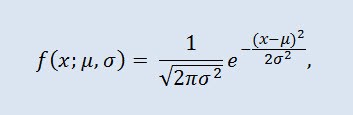
여기서 모수 μ는 랜덤 변수의 평균(기대치)이며 분포 밀도 곡선의 최대 좌표를 나타내며 σ²는 분산입니다.

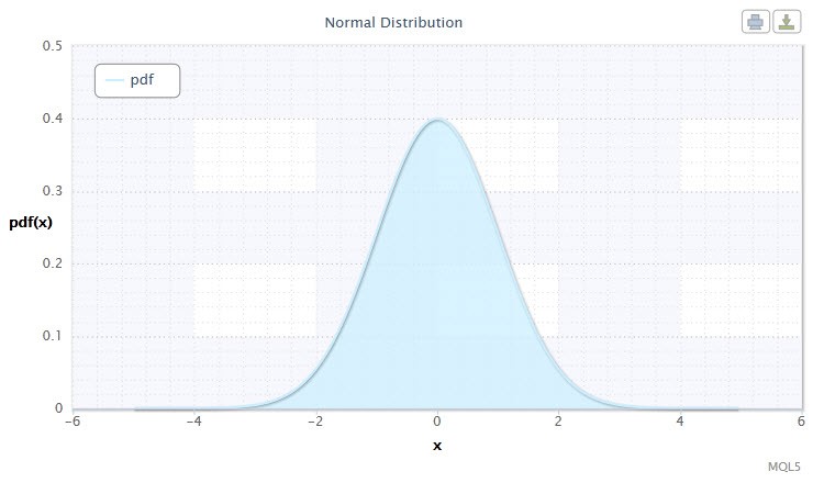
1번 그림. 정규 분포 밀도 Nor(0,1)

다음과 같은 식으로 표현됩니다: X ~ Nor(μ, σ²):

X 는 정규 분포 Nor에서 선택된 랜덤 변수;
μ 는 평균치 패러미터 (-∞ ≤ μ ≤ +∞);
σ 는 분산 패러미터 (0<σ).

랜덤 변수 X의 범위: -∞ ≤ X ≤ +∞.

이 문서에서 쓰인 공식은 다른 출처에서 쓰인 것과 약간 차이가 있을 수 있습니다. 그런 차이가 수학적으로 큰 차이가 있는 것은 아닙니다. 몇몇 경우 패러미터를 정할 때의 조건에 따른 것입니다.

정규 분포는 통계에서 중요한 역할을 하는데, 이는 많은 수의 랜덤 원인 사이의 교호작용으로 인해 발생하는 규칙성을 반영하며, 어느 것도 지배력을 가지지 않기 때문입니다. 그리고 비록 정규 분포가 금융 시장에서 드문 예이기는 하지만, 그럼에도 불구하고, 비정상의 정도와 성격을 결정하기 위해서는 그것을 경험적 분포와 비교하는 것이 중요합니다.

CNormaldist 클래스를 다음과 같이 정규 분포 로 정의합시다:

//+------------------------------------------------------------------+
//|                Normal Distribution class definition              |
//+------------------------------------------------------------------+
class CNormaldist : CErf // Erf class inheritance
  {
public:
   double            mu, //mean parameter (μ)
   sig;                 //variance parameter (σ)
   //+------------------------------------------------------------------+
   //| CNormaldist class constructor                                    |
   //+------------------------------------------------------------------+
   void  CNormaldist()
     {
      mu=0.0;sig=1.0; //default parameters μ and σ
      if(sig<=0.) Alert("bad sig in Normal Distribution!");
     }
   //+------------------------------------------------------------------+
   //| Probability density function (pdf)                               |
   //+------------------------------------------------------------------+
   double pdf(double x)
     {
      return(0.398942280401432678/sig)*exp(-0.5*pow((x-mu)/sig,2));
     }
   //+------------------------------------------------------------------+
   //| Cumulative distribution function (cdf)                           |
   //+------------------------------------------------------------------+
   double cdf(double x)
     {
      return 0.5*erfc(-0.707106781186547524*(x-mu)/sig);
     }
   //+------------------------------------------------------------------+
   //| Inverse cumulative distribution function (invcdf)                |
   //| quantile function                                                |
   //+------------------------------------------------------------------+
   double invcdf(double p)
     {
      if(!(p>0. && p<1.))
         Alert("bad p in Normal Distribution!");
      return -1.41421356237309505*sig*inverfc(2.*p)+mu;
     }
   //+------------------------------------------------------------------+
   //| Reliability (survival) function (sf)                             |
   //+------------------------------------------------------------------+
   double sf(double x)
     {
      return 1-cdf(x);
     }
  };

//+------------------------------------------------------------------+

보다시피, CNormaldist 클래스는 СErf 기본 클래스에서 파생되었으며 에러 함수 클래스를 정의합니다. 이는 CNormaldist 클래스 메소드 일부의 계산에 필요하게 됩니다. СErf 클래스와 보조 함수 erfcc는 이렇게 보입니다:

//+------------------------------------------------------------------+
//|                Error Function class definition                   |
//+------------------------------------------------------------------+
class CErf
  {
public:
   int               ncof;    // coefficient array size
   double            cof[28]; // Chebyshev coefficient array
   //+------------------------------------------------------------------+
   //| CErf class constructor                                           |
   //+------------------------------------------------------------------+
   void CErf()
     {
      int Ncof=28;
      double Cof[28]=//Chebyshev coefficients
        {
         -1.3026537197817094,6.4196979235649026e-1,
         1.9476473204185836e-2,-9.561514786808631e-3,-9.46595344482036e-4,
         3.66839497852761e-4,4.2523324806907e-5,-2.0278578112534e-5,
         -1.624290004647e-6,1.303655835580e-6,1.5626441722e-8,-8.5238095915e-8,
         6.529054439e-9,5.059343495e-9,-9.91364156e-10,-2.27365122e-10,
         9.6467911e-11, 2.394038e-12,-6.886027e-12,8.94487e-13, 3.13092e-13,
         -1.12708e-13,3.81e-16,7.106e-15,-1.523e-15,-9.4e-17,1.21e-16,-2.8e-17
        };
      setCErf(Ncof,Cof);
     };
   //+------------------------------------------------------------------+
   //| Set-method for ncof                                              |
   //+------------------------------------------------------------------+
   void setCErf(int Ncof,double &Cof[])
     {
      ncof=Ncof;
      ArrayCopy(cof,Cof);
     };
   //+------------------------------------------------------------------+
   //| CErf class destructor                                            |
   //+------------------------------------------------------------------+
   void ~CErf(){};
   //+------------------------------------------------------------------+
   //| Error function                                                   |
   //+------------------------------------------------------------------+
   double erf(double x)
     {
      if(x>=0.0) return 1.0-erfccheb(x);
      else return erfccheb(-x)-1.0;
     }
   //+------------------------------------------------------------------+
   //| Complementary error function                                     |
   //+------------------------------------------------------------------+
   double erfc(double x)
     {
      if(x>=0.0) return erfccheb(x);
      else return 2.0-erfccheb(-x);
     }
   //+------------------------------------------------------------------+
   //| Chebyshev approximations for the error function                  |
   //+------------------------------------------------------------------+
   double erfccheb(double z)
     {
      int j;
      double t,ty,tmp,d=0.0,dd=0.0;
      if(z<0.) Alert("erfccheb requires nonnegative argument!");
      t=2.0/(2.0+z);
      ty=4.0*t-2.0;
      for(j=ncof-1;j>0;j--)
        {
         tmp=d;
         d=ty*d-dd+cof[j];
         dd=tmp;
        }
      return t*exp(-z*z+0.5*(cof[0]+ty*d)-dd);
     }
   //+------------------------------------------------------------------+
   //| Inverse complementary error function                             |
   //+------------------------------------------------------------------+
   double inverfc(double p)
     {
      double x,err,t,pp;
      if(p >= 2.0) return -100.0;
      if(p <= 0.0) return 100.0;
      pp=(p<1.0)? p : 2.0-p;
      t = sqrt(-2.*log(pp/2.0));
      x = -0.70711*((2.30753+t*0.27061)/(1.0+t*(0.99229+t*0.04481)) - t);
      for(int j=0;j<2;j++)
        {
         err=erfc(x)-pp;
         x+=err/(M_2_SQRTPI*exp(-pow(x,2))-x*err);
        }
      return(p<1.0? x : -x);
     }
   //+------------------------------------------------------------------+
   //| Inverse error function                                           |
   //+------------------------------------------------------------------+
   double inverf(double p)
     {return inverfc(1.0-p);}
  };
//+------------------------------------------------------------------+
double erfcc(const double x)
/* 
 complementary error function erfc(x) with
 a relative error of 1.2 * 10^(-7)               
*/
  {
   double t,z=fabs(x),ans;
   t=2./(2.0+z);
   ans=t*exp(-z*z-1.26551223+t*(1.00002368+t*(0.37409196+t*(0.09678418+
             t*(-0.18628806+t*(0.27886807+t*(-1.13520398+t*(1.48851587+
             t*(-0.82215223+t*0.17087277)))))))));
   return(x>=0.0 ? ans : 2.0-ans);
  }
//+------------------------------------------------------------------+

2.1.2 로그-정규 분포

이제 로그-정규 분포를 살펴봅시다.

확률 이론에서 로그-정규 분포는 절대 연속 분포의 2-모수 군입니다. 랜덤 변수가 로그-정규 분포를 따르는 경우 그 변수의 로그가 정규 분포가 됩니다.

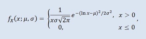
μ 는 위치 패러미터 (0<μ ), 그리고 σ 는 배율 패러미터 (0<σ).

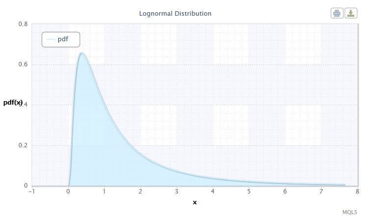
2번 그림. 로그-정규 분포 밀도 Logn(0,1)

다음과 같은 포맷으로 표현됩니다: X ~ Logn(μ, σ²):

X 는 로그-정규 분포 Logn에서 선택된 랜덤 변수;
μ 는 위치 패러미터입니다 (0<μ );
σ 는 배율 패러미터입니다 (0<σ).

랜덤 변수 X의 범위: 0 ≤ X ≤ +∞.

로그-정규 분포를 설명하는 CLognormaldist 클래스를 만듭시다 . 아래처럼 보일 것입니다:

//+------------------------------------------------------------------+
//|                Lognormal Distribution class definition           |
//+------------------------------------------------------------------+
class CLognormaldist : CErf // Erf class inheritance
  {
public:
   double            mu, //location parameter (μ)
   sig;                 //scale parameter (σ)
   //+------------------------------------------------------------------+
   //| CLognormaldist class constructor                                 |
   //+------------------------------------------------------------------+
   void  CLognormaldist()
     {
      mu=0.0;sig=1.0; //default parameters μ and σ
      if(sig<=0.) Alert("bad sig in Lognormal Distribution!");
     }
   //+------------------------------------------------------------------+
   //| Probability density function (pdf)                               |
   //+------------------------------------------------------------------+
   double pdf(double x)
     {
      if(x<0.) Alert("bad x in Lognormal Distribution!");
      if(x==0.) return 0.;
      return(0.398942280401432678/(sig*x))*exp(-0.5*pow((log(x)-mu)/sig,2));
     }
   //+------------------------------------------------------------------+
   //| Cumulative distribution function (cdf)                           |
   //+------------------------------------------------------------------+
   double cdf(double x)
     {
      if(x<0.) Alert("bad x in Lognormal Distribution!");
      if(x==0.) return 0.;
      return 0.5*erfc(-0.707106781186547524*(log(x)-mu)/sig);
     }
   //+------------------------------------------------------------------+
   //| Inverse cumulative distribution function (invcdf)(quantile)      |
   //+------------------------------------------------------------------+
   double invcdf(double p)
     {
      if(!(p>0. && p<1.))
         Alert("bad p in Lognormal Distribution!");
      return exp(-1.41421356237309505*sig*inverfc(2.*p)+mu);
     }
   //+------------------------------------------------------------------+
   //| Reliability (survival) function (sf)                             |
   //+------------------------------------------------------------------+
   double sf(double x)
     {
      return 1-cdf(x);
     }
  };
//+------------------------------------------------------------------+

보시다시피 로그-정규 분포는 정규 분포와 그다지 다르지 않습니다. 차이는 패러미터 x가 log(x)로 바뀐 것 정도입니다.

2.1.3 코시 분포

확률 이론의 코시 분포(물리학에서는 로렌츠 분포 또는 브라이트-위그너 분포라고도 함)는 절대 연속 분포의 클래스입니다. 코시 분산 랜덤 변수는 기대치도 분산도 없는 변수의 일반적인 예입니다. 밀도는 다음의 형태로 표현됩니다:

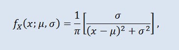
μ 는 위치 패러미터이며 (-∞ ≤ μ ≤ +∞ ), 그리고 σ 는 배율 패러미터입니다 (0<σ).

코시 분포의 표현은 다음과 같이 이루어집니다: X ~ Cau(μ, σ):

X 는 코시 분포 Cau에서 선택된 랜덤 변수입니다;
μ 는 위치 패러미터입니다 (-∞ ≤ μ ≤ +∞ );
σ 는 배율 패러미터입니다 (0<σ).

랜덤 변수 X의 범위: -∞ ≤ X ≤ +∞.

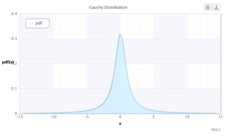
3번 그림. 코시 분포 밀도 Cau(0,1)

CCauchydist 클래스를 이용해 MQL5 포맷으로 만들어지면 이렇게 보입니다:

//+------------------------------------------------------------------+
//|                Cauchy Distribution class definition              |
//+------------------------------------------------------------------+
class CCauchydist //
  {
public:
   double            mu,//location parameter (μ)
   sig;                 //scale parameter (σ)
   //+------------------------------------------------------------------+
   //| CCauchydist class constructor                                    |
   //+------------------------------------------------------------------+
   void  CCauchydist() 
     {
      mu=0.0;sig=1.0; //default parameters μ and σ
      if(sig<=0.) Alert("bad sig in Cauchy Distribution!");
     }
   //+------------------------------------------------------------------+
   //| Probability density function (pdf)                               |
   //+------------------------------------------------------------------+
   double pdf(double x)
     {
      return 0.318309886183790671/(sig*(1.+pow((x-mu)/sig,2)));
     }
   //+------------------------------------------------------------------+
   //| Cumulative distribution function (cdf)                           |
   //+------------------------------------------------------------------+
   double cdf(double x)
     {
      return 0.5+0.318309886183790671*atan2(x-mu,sig); //todo      
     }
   //+------------------------------------------------------------------+
   //| Inverse cumulative distribution function (invcdf) (quantile func)|
   //+------------------------------------------------------------------+
   double invcdf(double p)
     {
      if(!(p>0. && p<1.))
         Alert("bad p in Cauchy Distribution!");
      return mu+sig*tan(M_PI*(p-0.5));
     }
   //+------------------------------------------------------------------+
   //| Reliability (survival) function (sf)                             |
   //+------------------------------------------------------------------+
   double sf(double x)
     {
      return 1-cdf(x);
     }
  };
//+------------------------------------------------------------------+

하나 말하고 싶은 것은 atan2()함수가 이용되었다는 것으로 이 함수는 아크탄젠트 값을 라디안으로 반환합니다:

double atan2(double y,double x)
/*
 Returns the principal value of the arc tangent of y/x,
 expressed in radians. To compute the value, the function 
 uses the sign of both arguments to determine the quadrant.
 y - double value representing an y-coordinate.
 x - double value representing an x-coordinate. 
*/
  {
   double a;
   if(fabs(x)>fabs(y))
      a=atan(y/x);
   else
     {
      a=atan(x/y); // pi/4 <= a <= pi/4
      if(a<0.)
         a=-1.*M_PI_2-a; //a is negative, so we're adding
      else
         a=M_PI_2-a;
     }
   if(x<0.)
     {
      if(y<0.)
         a=a-M_PI;
      else
         a=a+M_PI;
     }
   return a;
  }

2.1.4 쌍곡 시컨트 분포

쌍곡 시컨트 분포 는 금융 랭크 분석에 관심있으신 분들이 흥미롭게 보실만 합니다.

확률 이론과 통계에서, 쌍곡선 시컨트 분포는 확률 밀도 함수와 특성 함수가 쌍곡선 구간 함수에 비례하는 연속 확률 분포입니다. 밀도는 이하의 공식으로 구해집니다:

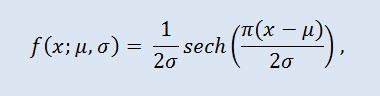
μ 는 위치 패러미터이며 (-∞ ≤ μ ≤ +∞ ), 그리고 σ 는 배율 패러미터입니다 (0<σ).

4번 그림. 쌍곡 시컨트 분포 밀도 HS(0,1)

이 표현은 다음의 포맷으로 이루어집니다: X ~ HS(μ, σ):

X 는 랜덤 변수입니다;
μ 는 위치 패러미터입니다 (-∞ ≤ μ ≤ +∞ );
σ 는 배율 패러미터입니다 (0<σ).

랜덤 변수 X의 범위: -∞ ≤ X ≤ +∞.

다음처럼 CHypersecdist 클래스를 활용하여 설명해봅시다:

//+------------------------------------------------------------------+
//|        Hyperbolic Secant Distribution class definition           |
//+------------------------------------------------------------------+
class CHypersecdist //
  {
public:
   double            mu,// location parameter (μ)
   sig;                 //scale parameter (σ)
   //+------------------------------------------------------------------+
   //| CHypersecdist class constructor                                 |
   //+------------------------------------------------------------------+
   void  CHypersecdist()
     {
      mu=0.0;sig=1.0; //default parameters μ and σ
      if(sig<=0.) Alert("bad sig in Hyperbolic Secant Distribution!");
     }
   //+------------------------------------------------------------------+
   //| Probability density function (pdf)                               |
   //+------------------------------------------------------------------+
   double pdf(double x)
     {
      return sech((M_PI*(x-mu))/(2*sig))/2*sig;
     }
   //+------------------------------------------------------------------+
   //| Cumulative distribution function (cdf)                           |
   //+------------------------------------------------------------------+
   double cdf(double x)
     {
      return 2/M_PI*atan(exp((M_PI*(x-mu)/(2*sig))));
     }
   //+------------------------------------------------------------------+
   //| Inverse cumulative distribution function (invcdf) (quantile func)|
   //+------------------------------------------------------------------+
   double invcdf(double p)
     {
      if(!(p>0. && p<1.))
         Alert("bad p in Hyperbolic Secant Distribution!");
      return(mu+(2.0*sig/M_PI*log(tan(M_PI/2.0*p))));
     }
   //+------------------------------------------------------------------+
   //| Reliability (survival) function (sf)                             |
   //+------------------------------------------------------------------+
   double sf(double x)
     {
      return 1-cdf(x);
     }
  };
//+------------------------------------------------------------------+

확률 밀도 함수가 쌍곡선 시컨트 함수에 비례하는 쌍곡선 시컨트 함수에서 이 분포의 이름을 얻었다고 보는 것은 쉬운 예상입니다.

쌍곡 시컨트 함수 sech 는 이하와 같습니다:

//+------------------------------------------------------------------+
//|              Hyperbolic Secant Function                          |
//+------------------------------------------------------------------+
double sech(double x)
// Hyperbolic Secant Function
  {
   return 2/(pow(M_E,x)+pow(M_E,-x));
  }

2.1.5 스튜던트 t 분포

스튜던트 t 분포는 통계학에서 중요한 분포입니다.

확률 이론에서 스튜던트 t 분포는 대부분 절대 연속 분포의 단일 모수 군이다. 그러나 분포 밀도 함수에 의해 주어진 3-모수 분포로도 간주할 수 있습니다.

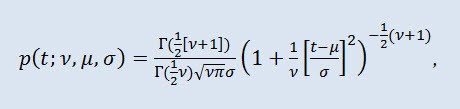
Г 는 오일러 감마 함수, ν 는 형상 패러미터 (ν>0), μ 는 위치 패러미터이며 (-∞ ≤ μ ≤ +∞ ), σ 는 배율 패러미터입니다 (0<σ).

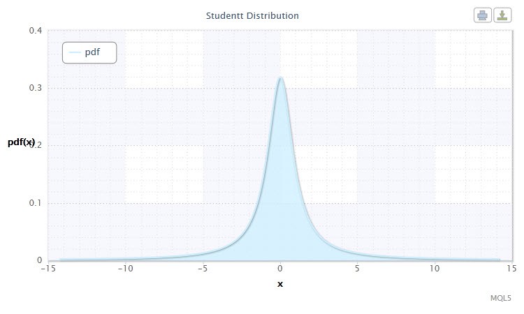
5번 그림. 스튜던트 t 분포 밀도 Stt(1,0,1)

이 표현은 다음의 형식을 따릅니다: t ~ Stt(ν,μ,σ), where:

t 는 스튜던트의 t 분산 Stt에서 선택된 랜덤 변수입니다;
ν 는 형태 패러미터입니다 (ν>0)
μ 는 위치 패러미터입니다 (-∞ ≤ μ ≤ +∞ );
σ 는 배율 패러미터입니다 (0<σ).

랜덤 변수 X의 범위: -∞ ≤ X ≤ +∞.

특히 가설 검정에서 표준 t-분포는 μ=0 및 σ=1과 함께 사용되는 경우가 많습니다. 따라서 모수 v를 갖는 단일 모수 분포로 변합니다.

이 분포는 종종 기대값 가설, 회귀 관계 계수, 동질성 가설 등을 테스트할 때 신뢰 구간을 통해 기대값, 추정값 및 기타 특성을 추정하는 데 사용됩니다.

스튜던트 분포를 CStudenttdist 클래스를 통해 설명해봅시다:

//+------------------------------------------------------------------+
//|                Student's t-distribution class definition         |
//+------------------------------------------------------------------+
class CStudenttdist : CBeta // CBeta class inheritance
  {
public:
   int               nu;     // shape parameter (ν)
   double            mu,     // location parameter (μ)
   sig,                     // scale parameter (σ)
   np,                      // 1/2*(ν+1)
   fac;                     // Г(1/2*(ν+1))-Г(1/2*ν)
   //+------------------------------------------------------------------+
   //| CStudenttdist class constructor                                  |
   //+------------------------------------------------------------------+
   void  CStudenttdist()
     {
      int Nu=1;double Mu=0.0,Sig=1.0; //default parameters ν, μ and σ
      setCStudenttdist(Nu,Mu,Sig);
     }
   void setCStudenttdist(int Nu,double Mu,double Sig)
     {
      nu=Nu;
      mu=Mu;
      sig=Sig;
      if(sig<=0. || nu<=0.) Alert("bad sig,nu in Student-t Distribution!");
      np=0.5*(nu+1.);
      fac=gammln(np)-gammln(0.5*nu);
     }
   //+------------------------------------------------------------------+
   //| Probability density function (pdf)                               |
   //+------------------------------------------------------------------+
   double pdf(double x)
     {
      return exp(-np*log(1.+pow((x-mu)/sig,2.)/nu)+fac)/(sqrt(M_PI*nu)*sig);
     }
   //+------------------------------------------------------------------+
   //| Cumulative distribution function (cdf)                           |
   //+------------------------------------------------------------------+
   double cdf(double t)
     {
      double p=0.5*betai(0.5*nu,0.5,nu/(nu+pow((t-mu)/sig,2)));
      if(t>=mu) return 1.-p;
      else return p;
     }
   //+------------------------------------------------------------------+
   //| Inverse cumulative distribution function (invcdf) (quantile func)|
   //+------------------------------------------------------------------+
   double invcdf(double p)
     {
      if(p<=0. || p>=1.) Alert("bad p in Student-t Distribution!");
      double x=invbetai(2.*fmin(p,1.-p),0.5*nu,0.5);
      x=sig*sqrt(nu*(1.-x)/x);
      return(p>=0.5? mu+x : mu-x);
     }
   //+------------------------------------------------------------------+
   //| Reliability (survival) function (sf)                             |
   //+------------------------------------------------------------------+
   double sf(double x)
     {
      return 1-cdf(x);
     }
   //+------------------------------------------------------------------+
   //| Two-tailed cumulative distribution function (aa) A(t|ν)          |
   //+------------------------------------------------------------------+
   double aa(double t)
     {
      if(t < 0.) Alert("bad t in Student-t Distribution!");
      return 1.-betai(0.5*nu,0.5,nu/(nu+pow(t,2.)));
     }
   //+------------------------------------------------------------------+
   //| Inverse two-tailed cumulative distribution function (invaa)      |
   //| p=A(t|ν)                                                         |
   //+------------------------------------------------------------------+
   double invaa(double p)
     {
      if(!(p>=0. && p<1.)) Alert("bad p in Student-t Distribution!");
      double x=invbetai(1.-p,0.5*nu,0.5);
      return sqrt(nu*(1.-x)/x);
     }
  };
//+------------------------------------------------------------------+

CStudenttdist 클래스 리스트는 CBeta가 기반 클래스이며 불완전한 베타 함수를 다루는 것을 보여줍니다.

CBeta 클래스는 다음과 같이 보입니다:

//+------------------------------------------------------------------+
//|            Incomplete Beta Function class definition             |
//+------------------------------------------------------------------+
class CBeta : public CGauleg18
  {
private:
   int               Switch;                     //when to use the quadrature method
   double            Eps,Fpmin;
public:
   //+------------------------------------------------------------------+
   //| CBeta class constructor                                          |
   //+------------------------------------------------------------------+
   void CBeta()
     {
      int swi=3000;
      setCBeta(swi,EPS,FPMIN);
     };
   //+------------------------------------------------------------------+
   //| CBeta class set-method                                           |
   //+------------------------------------------------------------------+
   void setCBeta(int swi,double eps,double fpmin)
     {
      Switch=swi;
      Eps=eps;
      Fpmin=fpmin;
     };
   double            betai(const double a,const double b,const double x); //incomplete beta function Ix(a,b)
   double            betacf(const double a,const double b,const double x);//continued fraction for incomplete beta function
   double            betaiapprox(double a,double b,double x); //Incomplete beta by quadrature
   double            invbetai(double p,double a,double b);    //Inverse of incomplete beta function
  };

이 클래스는 또한 CGauleg18클래스를 기반으로 두고 있으며 이 클래스는 가우스-르장드르 사분법같은 수치적분법에 대한 계수를 제공합니다.

2.1.6 로그분포

저는 로그 분포를 다음 순서로 다루는 것을 추천드립니다.

확률 이론과 통계에서 로그 분포는 연속 확률 분포입니다. 이것의 누적 분포 함수는 로그 함수입니다. 모양은 정규 분포와 유사하지만 뒤로 갈 수록 더 무겁습니다. 분포 밀도:

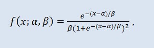
α 는 위치 패러미터 (-∞ ≤ α ≤ +∞ ), β 는 배율 패러미터 (0<β).

6번 그림 로그 분포 두께Logi(0,1)

표현은 다음과 같이 이루어집니다: X ~ Logi(α,β):

X 는 랜덤 변수입니다;
α 는 위치 패러미터입니다. (-∞ ≤ α ≤ +∞ );
β 는 배율 패러미터입니다 (0<β).

랜덤 변수 X의 범위: -∞ ≤ X ≤ +∞.

CLogisticdist 클래스가 상술한 분포의 구현입니다:

//+------------------------------------------------------------------+
//|                Logistic Distribution class definition            |
//+------------------------------------------------------------------+
class CLogisticdist
  {
public:
   double            alph,//location parameter (α)
   bet;                   //scale parameter (β)
   //+------------------------------------------------------------------+
   //| CLogisticdist class constructor                                  |
   //+------------------------------------------------------------------+
   void  CLogisticdist() 
     {
      alph=0.0;bet=1.0; //default parameters μ and σ
      if(bet<=0.) Alert("bad bet in Logistic Distribution!");
     }
   //+------------------------------------------------------------------+
   //| Probability density function (pdf)                               |
   //+------------------------------------------------------------------+
   double pdf(double x)
     {
      return exp(-(x-alph)/bet)/(bet*pow(1.+exp(-(x-alph)/bet),2));
     }
   //+------------------------------------------------------------------+
   //| Cumulative distribution function (cdf)                           |
   //+------------------------------------------------------------------+
   double cdf(double x)
     {
      double et=exp(-1.*fabs(1.81379936423421785*(x-alph)/bet));
      if(x>=alph) return 1./(1.+et);
      else return et/(1.+et);
     }
   //+------------------------------------------------------------------+
   //| Inverse cumulative distribution function (invcdf) (quantile func)|
   //+------------------------------------------------------------------+
   double invcdf(double p)
     {
      if(p<=0. || p>=1.) Alert("bad p in Logistic Distribution!");
      return alph+0.551328895421792049*bet*log(p/(1.-p));
     }
   //+------------------------------------------------------------------+
   //| Reliability (survival) function (sf)                             |
   //+------------------------------------------------------------------+
   double sf(double x)
     {
      return 1-cdf(x);
     }
  };
//+------------------------------------------------------------------+

2.1.7 지수분포

랜덤 변수의 지수 분포에 대해 알아봅시다.

랜덤 변수 X 는 밀도가 주어졌을 때 모수 λ > 0에서 지수 분포를 가집니다:

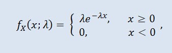
λ 는 배율 패러미터 (λ>0).

7번 그림. 지수 분포 밀도 Exp(1)

이는 아래와 같이 표현 가능합니다: X ~ Exp(λ):

X 는 랜덤 변수입니다;
λ 는 배율 패러미터입니다 (λ>0).

랜덤 변수 X의 범위: 0 ≤ X ≤ +∞.

이러한 분포는 특정 시간에 일어나는 일련의 사건을 하나씩 기술한다는 점에서 주목할 만합니다. 따라서, 트레이더는 이러한 분배를 사용하여 일련의 손실 거래 및 기타 정보를 분석할 수 있습니다.

MQL5 코드에서는 이 분포는 CExpondist 클래스를 통해 처리됩니다:

//+------------------------------------------------------------------+
//|                Exponential Distribution class definition         |
//+------------------------------------------------------------------+
class CExpondist
  {
public:
   double            lambda;   //scale parameter (λ)
   //+------------------------------------------------------------------+
   //| CExpondist class constructor                                     |
   //+------------------------------------------------------------------+
   void  CExpondist()
     {
      lambda=1.0;              //default parameter λ
      if(lambda<=0.) Alert("bad lambda in Exponential Distribution!");
     }
   //+------------------------------------------------------------------+
   //| Probability density function (pdf)                               |
   //+------------------------------------------------------------------+
   double pdf(double x)
     {
      if(x<0.) Alert("bad x in Exponential Distribution!");
      return lambda*exp(-lambda*x);
     }
   //+------------------------------------------------------------------+
   //| Cumulative distribution function (cdf)                           |
   //+------------------------------------------------------------------+
   double cdf(double x)
     {
      if(x < 0.) Alert("bad x in Exponential Distribution!");
      return 1.-exp(-lambda*x);
     }
   //+------------------------------------------------------------------+
   //| Inverse cumulative distribution function (invcdf) (quantile func)|
   //+------------------------------------------------------------------+
   double invcdf(double p)
     {
      if(p<0. || p>=1.) Alert("bad p in Exponential Distribution!");
      return -log(1.-p)/lambda;
     }
   //+------------------------------------------------------------------+
   //| Reliability (survival) function (sf)                             |
   //+------------------------------------------------------------------+
   double sf(double x)
     {
      return 1-cdf(x);
     }
  };
//+------------------------------------------------------------------+

2.1.8 감마분포

저는 감마 분포를 다음 랜덤 변수 연속 분포의 타입으로 결정했습니다.

확률론에서 감마 분포는 절대 연속 확률 분포의 2-모수 군입니다. 만약 모수 α 이 정수라면 그런 감마 분포는 얼랑 분포라고 불리기도 합니다. 그 밀도는 다음을 통해 구해집니다:

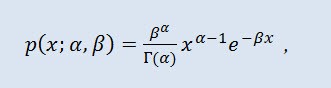
Г 는 오일러의 감마 함수이며, α는 형태 패러미터입니다 (0<α), β 는 배율 패러미터입니다 (0<β).

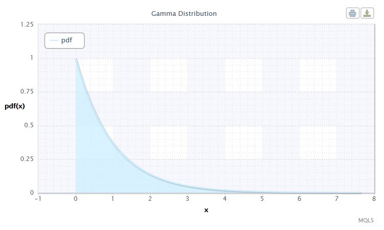
8번 그림. 감마 분포 두께 Gam(1,1).

다음과 같은 표현으로 나타낼 수 있습니다: X ~ Gam(α,β):

X 는 랜덤 변수입니다;
α 는 형태 패러미터입니다 (0<α);
β 는 배율 패러미터입니다 (0<β).

랜덤 변수 X의 범위: 0 ≤ X ≤ +∞.

CGammadist 클래스에서 정의된 변형은 다음과 같습니다:

//+------------------------------------------------------------------+
//|                Gamma Distribution class definition               |
//+------------------------------------------------------------------+
class CGammadist : CGamma // CGamma class inheritance
  {
public:
   double            alph,//continuous shape parameter (α>0)
   bet,                   //continuous scale parameter  (β>0)
   fac;                   //factor
   //+------------------------------------------------------------------+
   //| CGammaldist class constructor                                    |
   //+------------------------------------------------------------------+
   void  CGammadist()
     {
      setCGammadist();
     }
   void setCGammadist(double Alph=1.0,double Bet=1.0)//default parameters α and β
     {
      alph=Alph; bet=Bet;
      if(alph<=0. || bet<=0.) Alert("bad alph,bet in Gamma Distribution!");
      fac=alph*log(bet)-gammln(alph);
     }
   //+------------------------------------------------------------------+
   //| Probability density function (pdf)                               |
   //+------------------------------------------------------------------+
   double pdf(double x)
     {
      if(x<=0.) Alert("bad x in Gamma Distribution!");
      return exp(-bet*x+(alph-1.)*log(x)+fac);
     }
   //+------------------------------------------------------------------+
   //| Cumulative distribution function (cdf)                           |
   //+------------------------------------------------------------------+
   double cdf(double x)
     {
      if(x<0.) Alert("bad x in Gamma Distribution!");
      return gammp(alph,bet*x);
     }
   //+------------------------------------------------------------------+
   //| Inverse cumulative distribution function (invcdf) (quantile func)|
   //+------------------------------------------------------------------+
   double invcdf(double p)
     {
      if(p<0. || p>=1.) Alert("bad p in Gamma Distribution!");
      return invgammp(p,alph)/bet;
     }
   //+------------------------------------------------------------------+
   //| Reliability (survival) function (sf)                             |
   //+------------------------------------------------------------------+
   double sf(double x)
     {
      return 1-cdf(x);
     }
  };
//+------------------------------------------------------------------+

감마 분포는 CGamma 클래스에서 분화되었으며 이는 불완전 감마 함수를 다룹니다.

CGamma 클래스는 다음과 같이 정의되어 있습니다:

//+------------------------------------------------------------------+
//|            Incomplete Gamma Function class definition            |
//+------------------------------------------------------------------+
class CGamma : public CGauleg18
  {
private:
   int               ASWITCH;
   double            Eps,
   Fpmin,
   gln;
public:
   //+------------------------------------------------------------------+
   //| CGamma class constructor                                         |
   //+------------------------------------------------------------------+
   void CGamma()
     {
      int aswi=100;
      setCGamma(aswi,EPS,FPMIN);
     };
   void setCGamma(int aswi,double eps,double fpmin) //CGamma set-method
     {
      ASWITCH=aswi;
      Eps=eps;
      Fpmin=fpmin;
     };
   double            gammp(const double a,const double x); //incomplete gamma function
   double            gammq(const double a,const double x); //incomplete gamma function Q(a,x)
   void              gser(double &gamser,double a,double x,double &gln); //incomplete gamma function P(a,x)
   double            gcf(const double a,const double x); //incomplete gamma function Q(a,x)
   double            gammpapprox(double a,double x,int psig); //incomplete gamma by quadrature
   double            invgammp(double p,double a); //inverse of incomplete gamma function
  };
//+------------------------------------------------------------------+

CGamma 클래스와 CBeta 클래스 모두 CGauleg18가 기본 클래스입니다.

2.1.9 베타 분포

이제 베타 분포를 짚어봅시다.

확률 이론과 통계에서 베타 분포는 절대 연속 분포의 2-모수 군입니다. 유한한 간격으로 값이 정의되는 랜덤 변수를 설명하는 데 사용됩니다. 밀도는 다음과 같이 표현됩니다:

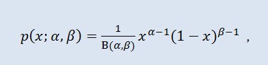
B 는베타 함수, α 는 첫번째 형상 패러미터 (0<α), β 는 두번째 형상 패러미터 (0<β).

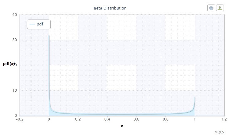
9번 그림. 베타 분산 밀도 Beta(0.5,0.5)

다음과 같이 표현됩니다: X ~ Beta(α,β):

X 는 랜덤 변수입니다;
α 는 첫번째 형태 패러미터입니다 (0<α);
β 는 두번째 형태 패러미터입니다 (0<β).

랜덤 변수 X의 범위: 0 ≤ X ≤ 1.

CBetadist 클래스가 베타 분산을 다음과 같이 다룹니다:

//+------------------------------------------------------------------+
//|                Beta Distribution class definition                |
//+------------------------------------------------------------------+
class CBetadist : CBeta // CBeta class inheritance
  {
public:
   double            alph,//continuous shape parameter (α>0)
   bet,                   //continuous shape parameter (β>0)
   fac;                   //factor
   //+------------------------------------------------------------------+
   //| CBetadist class constructor                                      |
   //+------------------------------------------------------------------+
   void  CBetadist()
     {
      setCBetadist();
     }
   void setCBetadist(double Alph=0.5,double Bet=0.5)//default parameters α and β
     {
      alph=Alph; bet=Bet;
      if(alph<=0. || bet<=0.) Alert("bad alph,bet in Beta Distribution!");
      fac=gammln(alph+bet)-gammln(alph)-gammln(bet);
     }
   //+------------------------------------------------------------------+
   //| Probability density function (pdf)                               |
   //+------------------------------------------------------------------+
   double pdf(double x)
     {
      if(x<=0. || x>=1.) Alert("bad x in Beta Distribution!");
      return exp((alph-1.)*log(x)+(bet-1.)*log(1.-x)+fac);
     }
   //+------------------------------------------------------------------+
   //| Cumulative distribution function (cdf)                           |
   //+------------------------------------------------------------------+
   double cdf(double x)
     {
      if(x<0. || x>1.) Alert("bad x in Beta Distribution");
      return betai(alph,bet,x);
     }
   //+------------------------------------------------------------------+
   //| Inverse cumulative distribution function (invcdf) (quantile func)|
   //+------------------------------------------------------------------+
   double invcdf(double p)
     {
      if(p<0. || p>1.) Alert("bad p in Beta Distribution!");
      return invbetai(p,alph,bet);
     }
   //+------------------------------------------------------------------+
   //| Reliability (survival) function (sf)                             |
   //+------------------------------------------------------------------+
   double sf(double x)
     {
      return 1-cdf(x);
     }
  };
//+------------------------------------------------------------------+

2.1.10 라플라스 분포

또 하나의 위대한 연속 분포는 라플라스 분포입니다 (이중 지수 분포).

확률 이론에서 라플라스 분포(이중 지수 분포)는 확률 밀도가 다음과 같은 랜덤 변수의 연속 분포입니다.

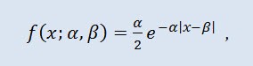
α 는 위치 패러미터 (-∞ ≤ α ≤ +∞ ), β 는 배율 패러미터 (0<β).

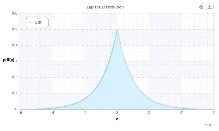
10번 그림. 라플라스 분산 밀도 Lap(0,1)

이는 다음과 같이 표현될 수 있습니다: X ~ Lap(α,β):

X 는 랜덤 변수입니다;
α 는 위치 패러미터입니다. (-∞ ≤ α ≤ +∞ );
β 는 배율 패러미터입니다 (0<β).

랜덤 변수 X의 범위: -∞ ≤ X ≤ +∞.

CLaplacedist 클래스는 이 목적을 위해 만들어졌습니다:

//+------------------------------------------------------------------+
//|                 Laplace Distribution class definition            |
//+------------------------------------------------------------------+
class CLaplacedist
  {
public:
   double            alph;   //location parameter (α)
   double            bet;    //scale parameter (β)
   //+------------------------------------------------------------------+
   //| CLaplacedist class constructor                                   |
   //+------------------------------------------------------------------+
   void  CLaplacedist()
     {
      alph=.0;               //default parameter α
      bet=1.;                //default parameter β
      if(bet<=0.) Alert("bad bet in Laplace Distribution!");
     }
   //+------------------------------------------------------------------+
   //| Probability density function (pdf)                               |
   //+------------------------------------------------------------------+
   double pdf(double x)
     {
      return exp(-fabs((x-alph)/bet))/2*bet;
     }
   //+------------------------------------------------------------------+
   //| Cumulative distribution function (cdf)                           |
   //+------------------------------------------------------------------+
   double cdf(double x)
     {
      double temp;
      if(x<0)
         temp=0.5*exp(-fabs((x-alph)/bet));
      else
         temp=1.-0.5*exp(-fabs((x-alph)/bet));
      return temp;
     }
   //+------------------------------------------------------------------+
   //| Inverse cumulative distribution function (invcdf) (quantile func)|
   //+------------------------------------------------------------------+
   double invcdf(double p)
     {
      double temp;
      if(p<0. || p>=1.) Alert("bad p in Laplace Distribution!");
      if(p<0.5)
         temp=bet*log(2*p)+alph;
      else
         temp=-1.*(bet*log(2*(1.-p))+alph);
      return temp;
     }
   //+------------------------------------------------------------------+
   //| Reliability (survival) function (sf)                             |
   //+------------------------------------------------------------------+
   double sf(double x)
     {
      return 1-cdf(x);
     }
  };
//+------------------------------------------------------------------+

MQL5 코드를 활용하여 10개의 연속 배포에 대해 10개의 클래스를 만들었습니다. 이것들 외에도, 예를 들어, 특정 기능과 방법 (예시, CBeta 및 CGamma)에 대한 필요성이 있었기 때문에 보완적인 몇 개의 클래스가 만들어졌습니다.

이제 이항 배포로 이동하여 이 분포 그룹에 대한 몇 가지 클래스를 생성하겠습니다.

2.2.1 이항 분포

이항분포로 시작해봅시다.

확률 이론에서 이항 분포는 모든 성공 확률이 동일한 독립 랜덤 실험 시퀀스의 성공 횟수에 대한 분포입니다. 확률 밀도는 다음 공식으로 구합니다:

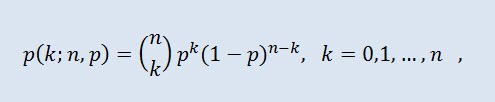
(n k) 는 이항 계수, n 는 시행 회수 (0 ≤ n), p 는 성공 확률 (0 ≤ p ≤1).

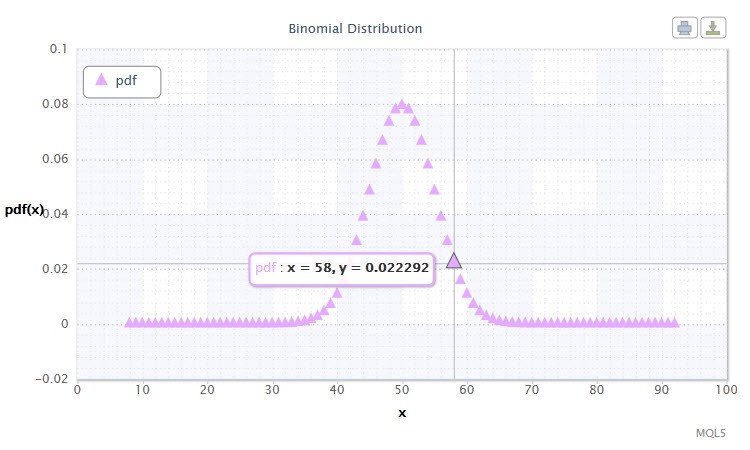
11번 그림. 이항 분포 밀도 Bin(100,0.5).

이는 다음과 같이 표현될 수 있습니다: k ~ Bin(n,p):

k 는 랜덤 변수입니다;
n 는 시도 회수입니다 (0 ≤ n);
p 는 성공 확률입니다 (0 ≤ p ≤1).

랜덤 변수 X의 범위: 0 or 1.

랜덤 변수 X의 가능한 값 범위가 당신에게는 어떤 의미를 가집니까? 실제로, 이러한 분포는 거래 시스템의 성공 (1) 및 실패 (0) 거래를 분석할때 도와주는 역할을 합니다.

СBinomialdist 클래스를 다음과 같이 만들어봅시다:

//+------------------------------------------------------------------+
//|               Binomial Distribution class definition             |
//+------------------------------------------------------------------+
class CBinomialdist : CBeta // CBeta class inheritance
  {
public:
   int               n;      //number of trials
   double            pe,     //success probability
   fac;                      //factor
   //+------------------------------------------------------------------+
   //| CBinomialdist class constructor                                  |
   //+------------------------------------------------------------------+
   void              CBinomialdist()
     {
      setCBinomialdist();
     }
   void setCBinomialdist(int N=100,double Pe=0.5)//default parameters n and pe
     {
      n=N; pe=Pe;
      if(n<=0 || pe<=0. || pe>=1.) Alert("bad args in Binomial Distribution!");
      fac=gammln(n+1.);
     }
   //+------------------------------------------------------------------+
   //| Probability density function (pdf)                               |
   //+------------------------------------------------------------------+
   double pdf(int k)
     {
      if(k<0) Alert("bad k in Binomial Distribution!");
      if(k>n) return 0.;
      return exp(k*log(pe)+(n-k)*log(1.-pe)+fac-gammln(k+1.)-gammln(n-k+1.));
     }
   //+------------------------------------------------------------------+
   //| Cumulative distribution function (cdf)                           |
   //+------------------------------------------------------------------+
   double cdf(int k)
     {
      if(k<0) Alert("bad k in Binomial Distribution!");
      if(k==0) return 0.;
      if(k>n) return 1.;
      return 1.-betai((double)k,n-k+1.,pe);
     }
   //+------------------------------------------------------------------+
   //| Inverse cumulative distribution function (invcdf) (quantile func)|
   //+------------------------------------------------------------------+
   int invcdf(double p)
     {
      int k,kl,ku,inc=1;
      if(p<=0. || p>=1.) Alert("bad p in Binomial Distribution!");
      k=fmax(0,fmin(n,(int)(n*pe)));
      if(p<cdf(k))
        {
         do
           {
            k=fmax(k-inc,0);
            inc*=2;
           }
         while(p<cdf(k));
         kl=k; ku=k+inc/2;
           } else {
         do
           {
            k=fmin(k+inc,n+1);
            inc*=2;
           }
         while(p>cdf(k));
         ku=k; kl=k-inc/2;
        }
      while(ku-kl>1)
        {
         k=(kl+ku)/2;
         if(p<cdf(k)) ku=k;
         else kl=k;
        }
      return kl;
     }
   //+------------------------------------------------------------------+
   //| Reliability (survival) function (sf)                             |
   //+------------------------------------------------------------------+
   double sf(int k)
     {
      return 1.-cdf(k);
     }
  };
//+------------------------------------------------------------------+

2.2.2 푸아송 분포

다음으로 검토할 분포는 푸아송 분포입니다.

푸아송 분포는 고정된 평균 강도로 서로 독립적으로 발생한다는 전제 하에 정해진 기간 동안 발생한 여러 사건들로 표현되는 랜덤 변수를 모델링한다. 밀도는 이하의 형태를 취합니다:

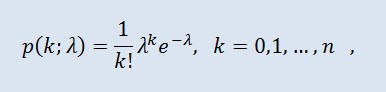
k! 는 팩토리얼이며, λ 는 위치 패러미터입니다 (0 < λ).

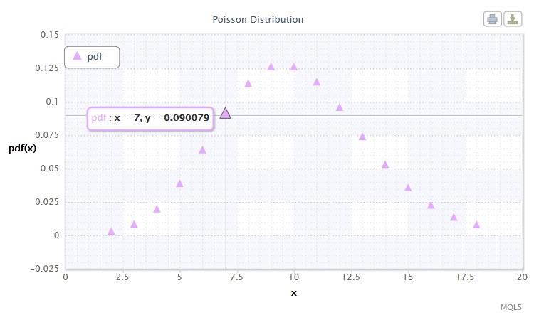
12번 그림. 푸아송 분포 밀도 Pois(10).

이는 다음과 같이 표현될 수 있습니다: k ~ Pois(λ),:

k 는 랜덤 변수입니다;
λ 는 위치 변수입니다 (0 < λ).

랜덤 변수 X의 범위: 0 ≤ X ≤ +∞.

푸아송 분포는 위험 정도를 추정할 때 중요한 "희귀 사건의 법칙"을 설명합니다.

CPoissondist 클래스가 이 작업을 처리합니다:

//+------------------------------------------------------------------+
//|               Poisson Distribution class definition              |
//+------------------------------------------------------------------+
class CPoissondist : CGamma // CGamma class inheritance
  {
public:
   double            lambda;   //location parameter (λ)
   //+------------------------------------------------------------------+
   //| CPoissondist class constructor                                   |
   //+------------------------------------------------------------------+
   void CPoissondist()
     {
      lambda=15.;
      if(lambda<=0.) Alert("bad lambda in Poisson Distribution!");
     }
   //+------------------------------------------------------------------+
   //| Probability density function (pdf)                               |
   //+------------------------------------------------------------------+
   double pdf(int n)
     {
      if(n<0) Alert("bad n in Poisson Distribution!");
      return exp(-lambda+n*log(lambda)-gammln(n+1.));
     }
   //+------------------------------------------------------------------+
   //| Cumulative distribution function (cdf)                           |
   //+------------------------------------------------------------------+
   double cdf(int n)
     {
      if(n<0) Alert("bad n in Poisson Distribution!");
      if(n==0) return 0.;
      return gammq((double)n,lambda);
     }
   //+------------------------------------------------------------------+
   //| Inverse cumulative distribution function (invcdf) (quantile func)|
   //+------------------------------------------------------------------+
   int invcdf(double p)
     {
      int n,nl,nu,inc=1;
      if(p<=0. || p>=1.) Alert("bad p in Poisson Distribution!");
      if(p<exp(-lambda)) return 0;
      n=(int)fmax(sqrt(lambda),5.);
      if(p<cdf(n))
        {
         do
           {
            n=fmax(n-inc,0);
            inc*=2;
           }
         while(p<cdf(n));
         nl=n; nu=n+inc/2;
           } else {
         do
           {
            n+=inc;
            inc*=2;
           }
         while(p>cdf(n));
         nu=n; nl=n-inc/2;
        }
      while(nu-nl>1)
        {
         n=(nl+nu)/2;
         if(p<cdf(n)) nu=n;
         else nl=n;
        }
      return nl;
     }
   //+------------------------------------------------------------------+
   //| Reliability (survival) function (sf)                             |
   //+------------------------------------------------------------------+
   double sf(int n)
     {
      return 1.-cdf(n);
     }
  };
//+=====================================================================+

문서 하나 안에서 모든 통계학적 분포를 다루는 것은 불가능하고, 필요하지도 않습니다. 사용자는 만약 원한다면 위에서 지정한 분포 갤러리를 확장할 수 있습니다. 만들어진 분포들은 Distribution_class.mqh 파일에서 확인할 수 있습니다.

3. 분포 그래프 생성하기

이제 우리가 만든 클래스가 향후 작업에 어떻게 활용될 수 있는지 알아보자고 제안합니다.

이 시점에서 다시 객체 지향 프로그래밍을 활용하여 저는 유저 지정 패러미터 분포를 처리하고 "HTML의 차트와 도표" 문서에 설명된대로 스크린 상에 표시하는 기능을 수행하는 CDistributionFigure 클래스를 작성했습니다..

//+------------------------------------------------------------------+
//|           Distribution Figure class definition                   |
//+------------------------------------------------------------------+
class CDistributionFigure
  {
private:
   Dist_type         type;  //distribution type
   Dist_mode         mode;  //distribution mode
   double            x;     //step start
   double            x11;   //left side limit
   double            x12;   //right side limit
   int               d;     //number of points
   double            st;    //step

public:
   double            xAr[]; //array of random variables
   double            p1[];  //array of probabilities
   void              CDistributionFigure();  //constructor 
   void              setDistribution(Dist_type Type,Dist_mode Mode,double X11,double X12,double St); //set-method
   void              calculateDistribution(double nn,double mm,double ss); //distribution parameter calculation
   void              filesave(); //saving distribution parameters
  };
//+------------------------------------------------------------------+

구현과정 생략. 이 클래스는 각각 Dist_type 및 Dist_mode에 대응되는 type 및 mode와 같은 데이터 멤버를 가지고 있는 점에 주목하시기 바랍니다. 이 타입들은 연구 중인 분포와 분포 타입의 열거들입니다.

자 이제 몇몇 분포에 대한 그래프틀 만들어 봅시다.

저는 연속 분산을 위한 스크립트로 continuousDistribution.mq5를 작성했고, 주요 라인은 아래와 같습니다:

//+------------------------------------------------------------------+
//|                     Input variables                              |
//+------------------------------------------------------------------+

input Dist_type dist;  //Distribution Type
input Dist_mode distM; //Distribution Mode
input int nn=1;        //Nu
input double mm=0.,    //Mu
            ss=1.;    //Sigma
//+------------------------------------------------------------------+
//| Script program start function                                    |
//+------------------------------------------------------------------+
void OnStart()
  {
//(Normal #0,Lognormal #1,Cauchy #2,Hypersec #3,Studentt #4,Logistic #5,Exponential #6,Gamma #7,Beta #8 , Laplace #9)
   double Xx1,      //left side limit
          Xx2,     //right side limit          
          st=0.05; //step
   if(dist==0) //Normal
     {
      Xx1=mm-5.0*ss/1.25;
      Xx2=mm+5.0*ss/1.25;
     }
   if(dist==2 || dist==4 || dist==5) //Cauchy,Studentt,Logistic
     {
      Xx1=mm-5.0*ss/0.35;
      Xx2=mm+5.0*ss/0.35;
     }
   else if(dist==1 || dist==6 || dist==7) //Lognormal,Exponential,Gamma
     {
      Xx1=0.001;
      Xx2=7.75;
     }
   else if(dist==8) //Beta
     {
      Xx1=0.0001;
      Xx2=0.9999;
      st=0.001;
     }
   else 
     {
      Xx1=mm-5.0*ss;
      Xx2=mm+5.0*ss;
     }
//---
   CDistributionFigure F;        //creation of the CDistributionFigure class instance 
   F.setDistribution(dist,distM,Xx1,Xx2,st);
   F.calculateDistribution(nn,mm,ss);
   F.filesave();
   string path=TerminalInfoString(TERMINAL_DATA_PATH)+"\\MQL5\\Files\\Distribution_function.htm";
   ShellExecuteW(NULL,"open",path,NULL,NULL,1);
  }
//+------------------------------------------------------------------+

이산 분포를 위하여 discreteDistribution.mq5 스크립트를 작성했습니다.

저는 코시 분산을 위한 표준 패러미터로 스크립트를 기동시켰고, 아래의 비디오에서 보실 수 있는 그래프를 얻었습니다.

마치며

이 문서에서는 MQL5에서도 코드화된 랜덤 변수의 몇 가지 이론적 분포를 다뤄봤습니다. 저는 시장거래 그 자체와 결과적으로 매매 시스템의 작업은 확률의 법칙에 기초해야 한다고 믿습니다.

이 문서가 그런 분야에 관심있으신 독자분들께 실질적인 도움이 되었기를 바랍니다. 저는 앞으로 이 주제에 대해 좀 더 자세히 살펴보고 확률 모델 분석에서 통계적 확률 분포가 어떻게 사용될 수 있는지를 보여주는 실제 사례를 제시하려합니다.

파일 위치:

#	파일	경로	설명
1	Distribution_class.mqh	%MetaTrader%\MQL5\Include	분포 클래스 갤러리
2	DistributionFigure_class.mqh	%MetaTrader%\MQL5\Include	분포 그래픽 표시 클래스
3	continuousDistribution.mq5	%MetaTrader%\MQL5\Scripts	연속 분포 생성 스크립트
4	discreteDistribution.mq5	%MetaTrader%\MQL5\Scripts	이산 분포 생성 스크립트
5	dataDist.txt	%MetaTrader%\MQL5\Files	분포 표시 데이터
6	Distribution_function.htm	%MetaTrader%\MQL5\Files	연속 분포 HTML 그래프
7	Distribution_function_discr.htm	%MetaTrader%\MQL5\Files	이산 분포 HTML 그래프
8	exporting.js	%MetaTrader%\MQL5\Files	그래프 익스포트용 JavaScript
9	highcharts.js	%MetaTrader%\MQL5\Files	JavaScript 라이브러리
10	jquery.min.js	%MetaTrader%\MQL5\Files	JavaScript 라이브러리

참조 문서:

K. Krishnamoorthy. Handbook of Statistical Distributions with Applications, Chapman and Hall/CRC 2006.
W.H. Press, et al. Numerical Recipes: The Art of Scientific Computing, Third Edition, Cambridge University Press: 2007. - 1256 pp.
S.V. Bulashev Statistics for Traders. - M.: Kompania Sputnik +, 2003. - 245 pp.
I. Gaidyshev Data Analysis and Processing: Special Reference Guide - SPb: Piter, 2001. - 752 pp.: ill.
A.I. Kibzun, E.R. Goryainova — Probability Theory and Mathematical Statistics. Basic Course with Examples and Problems
N.Sh. Kremer Probability Theory and Mathematical Statistics. M.: Unity-Dana, 2004. — 573 pp.

MetaQuotes 소프트웨어 사를 통해 러시아어가 번역됨.
원본 기고글: https://www.mql5.com/ru/articles/271

파일 첨부됨 |

ZIP파일 다운로드

distribution_class.mqh (108.26 KB)

continuousdistribution.mq5 (2.45 KB)

discretedistribution.mq5 (2.01 KB)

distribution_function.zip (59.99 KB)

distributionfigure_class.mqh (19.68 KB)

경고: 이 자료들에 대한 모든 권한은 MetaQuotes(MetaQuotes Ltd.)에 있습니다. 이 자료들의 전부 또는 일부에 대한 복제 및 재출력은 금지됩니다.

이 작가의 다른 글

토론으로 가기

소스 코드의 트레이싱, 디버깅, 및 구조 분석

실행된 코드의 구조 생성과 추적에 따른 전체 문제를 큰 어려움 없이 해결할 수 있습니다. MQL5 언어의 새로운 기능인 복잡한 유형의 데이터(구조 및 클래스)의 자동 생성과 로컬 범위를 벗어날 때 이러한 변수가 제거됨에 따라 MetaTrader 5에서 이러한 가능성이 대두되었습니다. 이 문서에서는 방법론에 대한 해석과 레디메이드 툴을 보여드리겠습니다.

선형 회귀 예시를 통한 인디케이터 가속 그 3가지 방법

이 문서에서는 인디케이터들의 메소드와 최적화 알고리즘에 대해 다루어볼 것입니다. 모든 독자분이 자신에게 적합한 메소드를 찾을 수 있을것입니다. 총 3개의 메소드가 다뤄집니다. 그 중 하나는 몹시 간단하며, 두번째 것은 탄탄한 수학적 지식을 필요로 하며 마지막 것은 약간 지혜가 필요합니다. 설명된 메소드 대부분을 이해하기 위해 인디케이터나 MetaTrader5 터미널 디자인 기능이 사용되었습니다. 이 메소드들은 매우 보편적이며 선형 회귀 계산의 가속뿐만 아니라 다른 많은 지표에도 사용할 수 있습니다.

통계적 추정

대부분의 수학적 모델과 방법은 서로 다른 가정을 기반으로 하기 때문에 시퀀스의 통계적 모수 추정은 매우 중요합니다. 예를 들어 분포 법칙의 정규성이나 분산 값 또는 기타 모수가 있습니다. 따라서 시계열 분석 및 예측 시 주요 통계 모수를 빠르고 명확하게 추정할 수 있는 간단하고 편리한 도구가 필요합니다. 이 문서는 랜덤 시퀀스의 가장 간단한 통계적 모수와 시각적 분석의 여러 메소드에 대해 설명할 것입니다. MQL5에서는 이러한 방법의 구현과 Gnuplot 애플리케이션을 사용한 계산 결과의 시각화 메소드를 제공합니다.

가격 상관 관계 통계 데이터를 기반으로 신호 필터링

과거 가격 변동과 미래의 트렌드 사이엔 어떠한 관계가 있을까요? 왜 오늘날의 가격이 과거에 했던 변동을 반복할까요? 통계학을 통하여 가격의 변동성을 예측할 수 있을까요? 답은, 맞다는 것입니다. 만약 아니라고 생각한다면 이 문서는 당신을 위한 것입니다. MQL5에서 거래 시스템에 대한 작동 필터를 만드는 방법을 알려드리겠습니다. 가격 변동에 대한 흥미로운 패턴을 보여줍니다.