Programming a Deep Neural Network from Scratch using MQL Language

Introduction

Since machine learning has recently gained popularity, many have heard about Deep Learning and desire to know how to apply it in the MQL language. I have seen simple implementations of artificial neurons with activation functions, but nothing that implements a real Deep Neural Network. In this article, I will introduce to you a Deep Neural Network implemented in the MQL language with its different activation functions, such as the hyperbolic tangent function for the hidden layers and the Softmax function for the output layer. We will move from the first step through the end to completely form the Deep Neural Network.

1. Making an Artificial Neuron

It begins with the basic unit of a neural network: a single neuron. In this article, I will concentrate on the different parts of the type of neuron that we are going to use in our Deep Neural Network, although the biggest difference between types of the neurons is usually the activation function.

1.1. Parts of a Single Neuron

The artificial neuron, loosely modeled off of a neuron in the human brain, simply hosts the mathematical computations. Like our neurons, it triggers when it encounters sufficient stimuli. The neuron combines input from the data with a set of coefficients, or weights, that either amplify or dampen that input, which thereby assigns significance to inputs for the task the algorithm is trying to learn. See each part of the neuron in action in the next image:

1.1.1. Inputs

The input is either an external trigger from the environment or comes from outputs of other artificial neurons; it is to be evaluated by the network. It serves as “food” for the neuron and passes through it, thereby becoming an output we can interpret due to the training we gave the neuron. They can be discrete values or real-valued numbers.

1.1.2. Weights

Weights are factors that are multiplied by the entries which correspond to them, increasing or decreasing their value, granting greater or lesser meaning to the input going inside the neuron and, therefore, to the output coming out. The goal of neural network training algorithms is to determine the "best" possible set of weight values for the problem to resolve.

1.1.3. Net Input Function

In this neuron part, the inputs and weights converge in a single-result product as the sum of the multiplication of each entry by its weight. This result or value is passed through the activation function, which then gives us the measures of influence that the input neuron has on the neural network output.

1.1.4. Activation Function

The activation function leads to the output. There can be several types of activation function (Sigmoid, Tan-h, Softmax, ReLU, among others). It decides whether or not a neuron should be activated. This article focuses on the Tan-h and Softmax types of function.

1.1.5. Output

Finally, we have the output. It can be passed to another neuron or sampled by the external environment. This value can be discrete or real, depending on the activation function used.

2. Building the Neural Network

The neural network is inspired by the information processing methods of biological nervous systems, such as the brain. It is composed of layers of artificial neurons, each layer connected to the next. Therefore, the previous layer acts as an input to the next layer, and so on to the output layer. The neural network's purpose could be clustering through unsupervised learning, classification through supervised learning or regression. In this article, we will focus on the ability to classify into three states: BUY, SELL or HOLD. Below is a neural network with one hidden layer:

3. Scaling from a Neural Network into a Deep Neural Network

What distinguishes a Deep Neural Network from the more commonplace single-hidden-layer neural networks is the number of layers that compose its depth. More than three layers (including input and output) qualifies as “deep” learning. Deep, therefore, is a strictly defined, technical term that means more than one hidden layer. The further you advance into the neural net, the more complex features there are that can be recognized by your neurons, since they aggregate and recombine features from the previous layer. It makes deep-learning networks capable of handling very large, high-dimensional data sets with billions of parameters that pass through nonlinear functions. In the image below, see a Deep Neural Network with 3 hidden layers:

3.1. Deep Neural Network Class

Now let's look at the class that we will use to create our neural network. The deep neural network is encapsulated in a program-defined class named DeepNeuralNetwork. The main method instantiates a 3-4-5-3 fully connected feed-forward neural network. Later, in a training session of the deep neural network in this article, I will show some examples of entries to feed our network, but for now we will focus on creating the network. The network is hard-coded for two hidden layers. Neural networks with three or more layers are very rare, but if you want to create a network with more layers you can do it easily by using the structure presented in this article. The input-to-layer-A weights are stored in matrix iaWeights, the layer-A-to-layer-B weights are stored in matrix abWeights, and the layer-B-to-output weights are stored in matrix boWeights. Since a multidimensional array can only be static or dynamic in the first dimension—with all further dimensions being static—the size of the matrix is declared as a constant variable using "#define" statement. I removed all using statements except the one that references the top-level System namespace to save space. You can find the complete source code in the attachments of the article.

Program structure:

#define SIZEI 4
#define SIZEA 5
#define SIZEB 3
//+------------------------------------------------------------------+
//|                                                                  |
//+------------------------------------------------------------------+
class DeepNeuralNetwork
  {
private:

   int               numInput;
   int               numHiddenA;
   int               numHiddenB;
   int               numOutput;

   double            inputs[];

   double            iaWeights[][SIZEI];
   double            abWeights[][SIZEA];
   double            boWeights[][SIZEB];

   double            aBiases[];
   double            bBiases[];
   double            oBiases[];

   double            aOutputs[];
   double            bOutputs[];
   double            outputs[];

public:

                     DeepNeuralNetwork(int _numInput,int _numHiddenA,int _numHiddenB,int _numOutput)
     {...}
     

   void SetWeights(double &weights[])
     {...}      
    

   void ComputeOutputs(double &xValues[],double &yValues[])
     {...}     
          

   double HyperTanFunction(double x)
     {...}      
     

   void Softmax(double &oSums[],double &_softOut[])
     {...}
      

  };
//+------------------------------------------------------------------+

The two hidden layers and the single output layer each have an array of associated bias values, named aBiases, bBiases and oBiases, respectively. The local outputs for the hidden layers are stored in class-scope arrays named aOutputs and bOutputs.

3.2. Computing Deep Neural Network Outputs

Method ComputeOutputs begins by setting up scratch arrays to hold preliminary (before activation) sums. Next, it computes the preliminary sum of weights times the inputs for the layer-A nodes, adds the bias values, then applies the activation function. Then, the layer-B local outputs are computed, using the just-computed layer-A outputs as local inputs and lastly, the final outputs are computed.

void ComputeOutputs(double &xValues[],double &yValues[])
     {
      double aSums[]; // hidden A nodes sums scratch array
      double bSums[]; // hidden B nodes sums scratch array
      double oSums[]; // output nodes sums

      ArrayResize(aSums,numHiddenA);
      ArrayFill(aSums,0,numHiddenA,0);
      ArrayResize(bSums,numHiddenB);
      ArrayFill(bSums,0,numHiddenB,0);
      ArrayResize(oSums,numOutput);
      ArrayFill(oSums,0,numOutput,0);

      int size=ArraySize(xValues);

      for(int i=0; i<size;++i) // copy x-values to inputs
         this.inputs[i]=xValues[i];

      for(int j=0; j<numHiddenA;++j) // compute sum of (ia) weights * inputs
         for(int i=0; i<numInput;++i)
            aSums[j]+=this.inputs[i]*this.iaWeights[i][j]; // note +=

      for(int i=0; i<numHiddenA;++i) // add biases to a sums
         aSums[i]+=this.aBiases[i];

      for(int i=0; i<numHiddenA;++i) // apply activation
         this.aOutputs[i]=HyperTanFunction(aSums[i]); // hard-coded

      for(int j=0; j<numHiddenB;++j) // compute sum of (ab) weights * a outputs = local inputs
         for(int i=0; i<numHiddenA;++i)
            bSums[j]+=aOutputs[i]*this.abWeights[i][j]; // note +=

      for(int i=0; i<numHiddenB;++i) // add biases to b sums
         bSums[i]+=this.bBiases[i];

      for(int i=0; i<numHiddenB;++i) // apply activation
         this.bOutputs[i]=HyperTanFunction(bSums[i]); // hard-coded

      for(int j=0; j<numOutput;++j) // compute sum of (bo) weights * b outputs = local inputs
         for(int i=0; i<numHiddenB;++i)
            oSums[j]+=bOutputs[i]*boWeights[i][j];

      for(int i=0; i<numOutput;++i) // add biases to input-to-hidden sums
         oSums[i]+=oBiases[i];

      double softOut[];
      Softmax(oSums,softOut); // softmax activation does all outputs at once for efficiency
      ArrayCopy(outputs,softOut);

      ArrayCopy(yValues,this.outputs);

     }

Behind the scenes, the neural network uses the hyperbolic tangent activation function (Tan-h) when computing the outputs of the two hidden layers, and the Softmax activation function when computing the final output values.

• Hyperbolic Tangent(Tan-h): Like the logistic Sigmoid, the Tan-h function is also sigmoidal, but instead outputs values that range (-1, 1). Thus, strongly negative inputs to the Tan-h will map to negative outputs. Additionally, only zero-valued inputs are mapped to near-zero outputs. In this case, I will show the mathematical formula but also its implementation in the MQL source code.

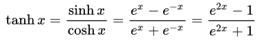
   double HyperTanFunction(double x)
     {
      if(x<-20.0) return -1.0; // approximation is correct to 30 decimals
      else if(x > 20.0) return 1.0;
      else return MathTanh(x); //Use explicit formula for MQL4 (1-exp(-2*x))/(1+exp(-2*x))
     }

• Softmax: Assigns decimal probabilities to each class in a case of multiple classes. Those decimal probabilities must add 1.0. This additional restriction allows the training to converge faster.

   void Softmax(double &oSums[],double &_softOut[])
     {
      // determine max output sum
      // does all output nodes at once so scale doesn't have to be re-computed each time
      int size=ArraySize(oSums);
      double max= oSums[0];
      for(int i = 0; i<size;++i)
         if(oSums[i]>max) max=oSums[i];

      // determine scaling factor -- sum of exp(each val - max)
      double scale=0.0;
      for(int i= 0; i<size;++i)
         scale+= MathExp(oSums[i]-max);

      ArrayResize(_softOut,size);
      for(int i=0; i<size;++i)
         _softOut[i]=MathExp(oSums[i]-max)/scale;

     }

4. Demo Expert Advisor using the DeepNeuralNetwork Class

Before starting to develop the Expert Advisor we must define the data that will be fed to our Deep Neural Network. Since a neural network is good at classifying patterns, we are going to use the relative values of a Japanese candle as input. These values would be the size of the upper shadow, body, lower shadow and direction of the candle (bullish or bearish). The number of entries does not necessarily have to be small but in this case it will suffice as a test program.

The demo Expert Advisor:

An structure 4-4-5-3 neural network requires a total of (4 * 4) + 4 + (4 * 5) + 5 + (5 * 3) + 3 = 63 weights and bias values.

#include <DeepNeuralNetwork.mqh> 

int numInput=4;
int numHiddenA = 4;
int numHiddenB = 5;
int numOutput=3;

DeepNeuralNetwork dnn(numInput,numHiddenA,numHiddenB,numOutput);


//--- weight & bias values
input double w0=1.0;
input double w1=1.0;
input double w2=1.0;
input double w3=1.0;
input double w4=1.0;
input double w5=1.0;
input double w6=1.0;
input double w7=1.0;
input double w8=1.0;
input double w9=1.0;
input double w10=1.0;
input double w11=1.0;
input double w12=1.0;
input double w13=1.0;
input double w14=1.0;
input double w15=1.0;
input double b0=1.0;
input double b1=1.0;
input double b2=1.0;
input double b3=1.0;
input double w40=1.0;
input double w41=1.0;
input double w42=1.0;
input double w43=1.0;
input double w44=1.0;
input double w45=1.0;
input double w46=1.0;
input double w47=1.0;
input double w48=1.0;
input double w49=1.0;
input double w50=1.0;
input double w51=1.0;
input double w52=1.0;
input double w53=1.0;
input double w54=1.0;
input double w55=1.0;
input double w56=1.0;
input double w57=1.0;
input double w58=1.0;
input double w59=1.0;
input double b4=1.0;
input double b5=1.0;
input double b6=1.0;
input double b7=1.0;
input double b8=1.0;
input double w60=1.0;
input double w61=1.0;
input double w62=1.0;
input double w63=1.0;
input double w64=1.0;
input double w65=1.0;
input double w66=1.0;
input double w67=1.0;
input double w68=1.0;
input double w69=1.0;
input double w70=1.0;
input double w71=1.0;
input double w72=1.0;
input double w73=1.0;
input double w74=1.0;
input double b9=1.0;
input double b10=1.0;
input double b11=1.0;

For inputs for our neural network we will use the following formula to determine which percentage represents each part of the candle, respecting the total of its size.

//+------------------------------------------------------------------+
//|percentage of each part of the candle respecting total size       |
//+------------------------------------------------------------------+
int CandlePatterns(double high,double low,double open,double close,double uod,double &xInputs[])
  {
   double p100=high-low;//Total candle size   
   double highPer=0;
   double lowPer=0;
   double bodyPer=0;
   double trend=0;

   if(uod>0)
     {
      highPer=high-close;
      lowPer=open-low;
      bodyPer=close-open;
      trend=1;

     }
   else
     {
      highPer=high-open;
      lowPer=close-low;
      bodyPer=open-close;
      trend=0;
     }
   if(p100==0)return(-1);
   xInputs[0]=highPer/p100;
   xInputs[1]=lowPer/p100;
   xInputs[2]=bodyPer/p100;
   xInputs[3]=trend;

   return(1);

  }

Now we can process the inputs through our neural network:

   MqlRates rates[];
   ArraySetAsSeries(rates,true);
   int copied=CopyRates(_Symbol,0,1,5,rates);

   //Compute the percent of the upper shadow, lower shadow and body in base of sum 100%
   int error=CandlePatterns(rates[0].high,rates[0].low,rates[0].open,rates[0].close,rates[0].close-rates[0].open,_xValues);

   if(error<0)return;
   
   dnn.SetWeights(weight);

   double yValues[];
   dnn.ComputeOutputs(_xValues,yValues);

Now the trading opportunity is processed-based on the neural network calculation. Remember, the Softmax function will produce 3 outputs based on the sum of 100%. The values are stored on the array "yValues" and the value with a number higher than 60% will be executed.

//--- if the output value of the neuron is mare than 60%
   if(yValues[0]>0.6)
     {
      if(m_Position.Select(my_symbol))//check if there is an open position
        {
         if(m_Position.PositionType()==POSITION_TYPE_SELL) m_Trade.PositionClose(my_symbol);//Close the opposite position if exists
         if(m_Position.PositionType()==POSITION_TYPE_BUY) return;
        }
      m_Trade.Buy(lot_size,my_symbol);//open a Long position
     }
//--- if the output value of the neuron is mare than 60%
   if(yValues[1]>0.6)
     {
      if(m_Position.Select(my_symbol))//check if there is an open position
        {
         if(m_Position.PositionType()==POSITION_TYPE_BUY) m_Trade.PositionClose(my_symbol);//Close the opposite position if exists
         if(m_Position.PositionType()==POSITION_TYPE_SELL) return;
        }
      m_Trade.Sell(lot_size,my_symbol);//open a Short position
     }

   if(yValues[2]>0.6)
     {
      m_Trade.PositionClose(my_symbol);//close any position

     }

5. Training the Deep Neural Network using strategy optimization

As you may have noticed, only the deep neural network feed-forward mechanism has been implemented, and it doesn't perform any training. This task is reserved for the strategy tester. Below, I show you how to train the neural network. Keep in mind, that due to a large number of inputs and the range of training parameters, it can only be trained in MetaTrader 5, but once the values of the optimization are obtained, it can easily be copied to MetaTrader 4.

The Strategy Tester configuration:

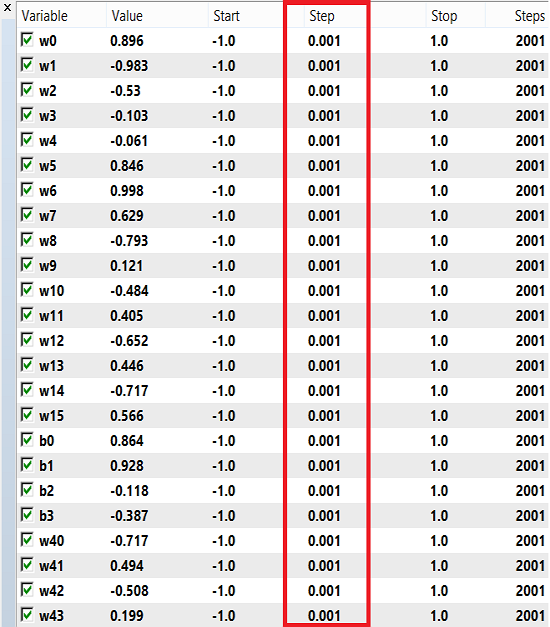
The weights and bias can use a range of numbers for training, from -1 to 1 and a step of 0.1, 0.01 or 0.001. You can try these values and see which one gets the best result. In my case, I have used 0.001 for the step as shown in the image below:

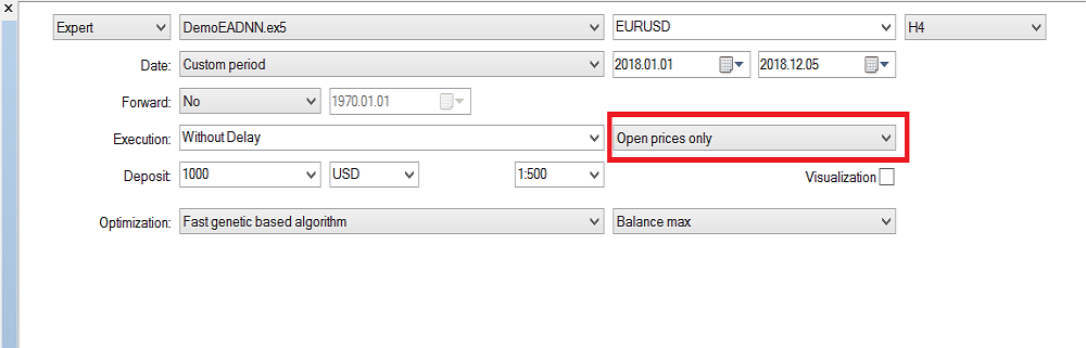
Please note that I have used "Open Prices Only" because I'm using the last closed candle, so it's not worth running it on every tick. Now I've been running the optimization on H4 time frame and for the last year I got this result on backtest:

Conclusion

The code and explanation presented in this article should give you a good basis for understanding neural networks with two hidden layers. What about three or more hidden layers? The consensus in research literature is that two hidden layers is sufficient for almost all practical problems. This article outlines an approach for developing improved models for exchange rate prediction using Deep Neural Networks, motivated by the ability of deep networks to learn abstract features from raw data. Preliminary results confirm that our deep network produces significantly higher predictive accuracy than the baseline models for developed currency markets.