Fractal Analysis of Joint Currency Movements

Introduction

You can often hear people discuss relationships between different currencies in the Forex market.

The main point at issue usually comes down to fundamental factors, hands-on experience or mere speculations resulting from personal stereotypes of the speaker. A hypothesis of one or more 'global' currencies 'dragging' all the rest can be considered the extreme case.

Indeed, what is the nature of relationships between various quotes? Are their movements coordinated or does the movement of one currency suggest nothing of the movement of another? The article describes an effort to tackle this issue using nonlinear dynamics and fractal geometry methods.

1. Theoretical Part

1.1. Dependent and independent variables

Let us have a look at two variables (quotes) x and y. At any given time, instantaneous values of these variables determine a point in the XY-plane (Fig. 1). Motion of the point in the course of time forms a trajectory. The form and type of such trajectory will depend on the type of relationship between the variables.

Figure 1. Point in the plane

For example, if the variable x has no relation to the variable y, you will observe no regular structure - the XY-plane will be uniformly filled with the points, provided their number is sufficient (Fig.2).

Figure 2. No correlation - uniformly filled plane

If however there is a relationship between x and y, a regular structure will appear, in the simplest case representing a curve (Fig. 3),

Figure 3. Presence of correlations - a curve

or even a more complex structure (Fig. 4).

Figure 4. Presence of correlations - a structure in the plane

The same is characteristic of a three- and more dimensional space: if all variables are interrelated or interdependent, the points will form a curve (Fig. 5), if there are two independent variables in a set, the points will form a surface (Fig. 6), in case of three independent variables, the points will fill the three-dimensional space, etc.

Figure 5. A curve in the three-dimensional space

Figure 6. A surface in the three-dimensional space

If there is no relationship between variables, the points will get uniformly distributed across all available dimensions (Fig. 7). Thus, we can speak about the nature of relationships between variables based on the way the points fill the space.

Figure 7. No correlation - points uniformly distributed in the space

The form of the resulting structure (line, surface, 3-D shape, etc.) is in this case of no importance.

What matters is a fractal dimension of that structure: 1 for sets describing lines, 2 for sets describing surfaces, 3 for sets describing volumes, etc. It is usually assumed that a fractal dimension value corresponds to the number of independent variables in a data set.

We can also come across a fractional dimension, e.g. 1.61 or 2.68. This may be the case if the resulting structure is a fractal i.e. a self-similar set of non-integral dimension. An example of a fractal is given in Figure 8, its dimension is approximately 1.89, i.e. this is no longer a line (dimension 1) and not yet a surface (dimension 2).

Figure 8. The Sierpinski carpet

A fractal dimension of one and the same set may be different at different scales.

For instance, if you take a look at the set in Figure 9 from 'afar', you will clearly see the line, i.e. a fractal dimension of the given set is 1. A 'close-up' look at the same set will no longer reveal a line but a 'fuzzy tube' where the points do not form a clear line but are accumulated around it in a random way. A fractal dimension of that 'tube' shall be equal to the dimension of the space in which our structure is considered as the points in the 'tube' will get uniformly distributed across all available dimensions.

An increase in fractal dimension at smaller scales allows to estimate a dimension at which the relationships between variables become indiscernible due to the presence of random noise.

Figure 9. Example of a fractal 'tube'

1.2. Estimating fractal dimension

A fractal dimension can be estimated using the box-counting method based on the analysis of dependence of the number of boxes containing points of a set on the side length of the box (it does not have to be a 3D box - a 'box' in the one-dimensional space will be represented by a segment, in the two-dimensional space by a square, etc.)

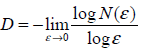
Theoretically, this dependence is given by N(ε)~1/ε^D, where D is the fractal dimension of the set, ε is the side length of the box, N(ε) – is the number of ε-sized boxes containing points of the set. It allows to estimate the fractal dimension

Without going into much detail, the operation of the algorithm can be described as follows:

1. A given set of points is broken down into ε-sized boxes and the number of boxes N containing at least one point of the set is counted.

2. For various ε a respective N value is determined, i.e. we accumulate data to plot the dependence N(ε).

3. The dependence N(ε) is plotted on double logarithmic coordinates where the slope of the dependence will correspond to the value of the fractal dimension.

For example, Figure 10 shows two sets: a plane figure (a) and a line (b). Cells that contain points of the set are filled in gray. Counting the number of 'gray' cells with different cell sizes, we obtain the dependences illustrated in Figure 11. The slope of the straight lines approximating these dependences helps estimate the fractal dimensions: Da≈2, Db≈1.

Figure 10. Measuring sets

Normally, a fractal dimension is estimated in practice using the Grassberger-Procaccia algorithm instead of the box-counting method, as it yields more accurate results in high-dimensional spaces. The idea of the algorithm is to obtain a dependence С(ε) of the probability of two points of a set getting into in a ε-sized cell on the cell size and to determine the slope of a linear section of such dependence.

Unfortunately, it is impossible to cover all aspects of estimating fractal dimension within the scope of this article. Further information, if required, can be found in specialized literature.

Figure 11. Estimated fractal dimension of sets

1.3. Example of estimating fractal dimension

To verify the performance of the proposed technique, let us determine the noise level and the number of independent variables for the set shown in Figure 9. This three-dimensional set consists of 3000 points and represents a line (one independent variable) with superimposed noise. The noise is normally distributed, with root-mean square error of 0.01.

Figure 12 demonstrates the dependence С(ε) in logarithmic scale. There are two linear sections intersecting at ε≈2^-4.6≈0.04. The slope of the first line is ≈2.6, the slope of the second line is ≈1.0.

The obtained results suggest that the test set has only one independent variable on the scale more than 0.0 and 'almost three' independent variables or superimposed noise on the scale less than 0.04. This is in good agreement with the initial data: according to the three-sigma rule, 99.7% of points form a 'tube' with a diameter of 2*3*0.01≈0.06.

Figure 12. Dependence C(e) in logarithmic scale

2. Practical Part

2.1. Initial data

Fractal properties of the Forex market were studied using public data covering the period from 2000 to 2009 inclusive. The study was performed on closing prices of seven major currency pairs: EURUSD, USDJPY, GBPUSD, AUDUSD, USDCHF, USDCAD, NZDUSD.

2.2. Implementation

Algorithms for estimating fractal dimension were implemented in the form of MATLAB environment functions based on developments made by Dr. Michael Small (http://www.eie.polyu.edu.hk/~ensmall/matlab/). Functions with implementation examples are available in the frac.rar archive attached to this article.

To speed up calculations, the most time-consuming part was written in C language. Before you start, compile the C function "interbin.c" using the MATLAB command "mex interbin.c".

2.3. Results of the study

Figure 13 shows a joint movement of EURUSD and GBPUSD prices from 2000 to 2010. The price values as such are demonstrated in Figures 14 and 15.

Figure 13. Joint movement of EURUSD and GBPUSD prices from 2000 to 2010

Figure 14. EURUSD price chart from 2000 to 2010

Figure 15. GBPUSD price chart from 2000 to 2010

A fractal dimension of the set shown in Figure 13 is approximately equal to 1.7 (Fig. 16). This means that EURUSD + GBPUSD movement does not represent a 'purely' random walk, otherwise its dimension would have been 2 (dimension of a random walk in two- and more-dimensional spaces is always equal to 2).

However, since the price movement is very similar to the random walk, we cannot analyze the price values by themselves - fractal dimension changes insignificantly when new currency pairs are added (Table 1) and it is impossible to draw any conclusion.

Currency pairs	EURUSD GBPUSD	+USDJPY	+AUDUSD	+USDCHF	+USDCAD	+NZDUSD
Dimension	1.7	1.9	1.9	1.9	1.9	1.9

Table 1. Change in dimension upon increase in the number of currencies

Figure 16. Estimated fractal dimension

To obtain more interesting results, we should proceed from the quotes to changes in them.

Dimension values for various increment intervals and different number of currency pairs are provided in Table 2.

	Dates	Number of points	EURUSD GBPUSD	+USDJPY	+AUDUSD	+USDCHF	+USDCAD	+NZDUSD
M5	14 Aug 2008 — 31 Dec 2009	100000	1.9	2.8	3.7	4.4	5.3	6.2
M15	18 Nov 2005 — 31 Dec 2009	100000	2	2.8	3.7	4.5	5.9	6.7
M30	16 Nov 2001 — 31 Dec 2009	100000	2	2.8	3.7	4.5	5.7	6.8
H1	03 Jan 2000 — 31 Dec 2009	61765	2	2.9	3.8	4.6	5.6	6.5
H4	03 Jan 2000 — 31 Dec 2009	15558	2	3	4	4.8	5.9	6.3
D1	03 Jan 2000 — 31 Dec 2009	2601	2	3	4	5.1	5.7	6.5

Table 2. Change in dimension at different increment intervals

If currencies are interrelated, the fractal dimension, every time the new currency pair is added, should increase less and less significantly to finally get to a certain value that will determine the number of 'free variables' in the currency exchange market.

If we also assume, that the 'market noise' is superimposed on prices, all available dimensions may get filled with the noise on short time frames (М5, М15, М30) and this effect should subside on longer time frames 'revealing' the dependences between the quotes (as in the test example).

As Table 2 suggests, this hypothesis was not confirmed by actual data: the set gets distributed across all available dimensions on all time frames, i.e. all currencies are independent of each other.

It is somewhat in conflict with intuitive assumptions regarding currency relationships. It appears that close currencies, e.g. GBP and CHF or AUD and NZD should exhibit similar dynamics. For example, Figure 17 shows increment dependences between NZDUSD and AUDUSD on M5 (correlation coefficient: 0.54) and D1 (correlation coefficient: 0.84) time frames.

Figure 17. Increment dependences between NZDUSD and AUDUSD on M5 (0.54) and D1 (0.84) time frames

As can be seen in this Figure, the dependence gets further and further stretched diagonally and the correlation coefficient value goes up as the interval increases. However, in terms of fractal dimension, the noise level is too high to consider such dependence a one-dimensional line. Fractal dimensions on longer intervals (weeks, months) will perhaps converge to a certain value but we are not given the facilities to check this due to insufficient number of points for estimation of the dimension.

Conclusion

It would certainly be more interesting to narrow down the movements of currencies to one or more independent variables to considerably simplify the task of reconstructing the market attractor and forecasting prices. The market however yields a different result: dependences are poorly pronounced and "well hidden" in a large amount of noise. The market is very efficient in this regard.

Methods of nonlinear dynamics that steadily yield good results in areas like medicine, physics, chemistry, biology and others, require particular attention and careful interpretation of findings when used in the market price analysis.

The obtained results do not expressly suggest the presence or absence of relationships between currencies. We can only say that the noise level on the given time frames is comparable to the 'strength' of the relationship so the question of relationships between currencies remains open.