Neural Additive Models for Fully Interpretable Signal Attribution in MQL5

Introduction

Every explainability technique applied to a trading model after the fact makes a promise it can't quite keep. SHAP values approximate what a black-box network is doing by perturbing inputs and averaging the effect. Partial dependence plots average over a background dataset and hope the interactions wash out. Both are useful, and both are guesses about a model whose real internal computation nobody can point to directly.

A Neural Additive Model (NAM) sidesteps the guessing entirely. Instead of one dense network where every input is tangled with every other input by the second layer, a NAM assigns each feature its own small subnetwork, and the final prediction is nothing more than the sum of what those subnetworks output. There is no approximation step because there is nothing to approximate — the contribution of feature i to the prediction is literally the output of subnetwork i. Plot it, and you are looking at the model's own internal arithmetic, not a reconstruction of it.

This article implements the architecture for MetaTrader 5. It trains a five-feature NAM in PyTorch, exports it to ONNX, and runs it in an Expert Advisor that reads both the signal and each feature's exact contribution on every closed bar. Three files ship with this article — an include class wrapping the ONNX model, the EA itself, and the Python training/export script — each walked through with its actual code below, not just described in prose.

Scope note: this article assumes familiarity with MQL5's ONNX integration (OnnxCreateFromBuffer, OnnxRun) and with training a small neural network in PyTorch. It does not re-derive backpropagation or ONNX's tensor format from scratch.

There's a practical reason this matters beyond intellectual tidiness. Most ML-driven EAs treat the model as a signal generator and stop there: a number comes out, a trade fires or doesn't, and the "why" lives nowhere except in whatever the training script's loss curve looked like weeks earlier. That's fine until the model starts behaving strangely on a live account, at which point the operator is debugging a black box with nothing but the inputs and the output to go on. A NAM exposes the middle of the chain: it shows how much each input moves the output and in which direction. It does so within the same forward pass, with no separate explainability step.

This does not remove standard caveats. A NAM still depends on feature quality, can overfit on small datasets, and requires out-of-sample checks of its shape functions before live use. What it removes is one specific failure mode: attribution that quietly stops matching the model the moment someone asks for it in detail.

Architecture and Mathematics

A generalized additive model, going back decades before neural networks were practical, predicts an outcome as a sum of one-dimensional functions, one per feature

g(y) = beta + f_1(x_1) + f_2(x_2) + ... + f_K(x_K)

where g is a link function (identity here, since the EA treats the output as a continuous directional signal rather than a probability) and each f_i is fit independently of the others, seeing only its own feature. Classically these f_i were splines or boosted trees. A Neural Additive Model replaces each f_i with a small neural network — expressive enough to learn a genuinely non-linear shape, but structurally forbidden from looking at any feature but its own.

That structural restriction is the entire point. A plain dense network with five inputs and one hidden layer will happily learn that RSI matters differently depending on what volume is doing — a real interaction, but one that makes "how much did RSI contribute" an ill-posed question. A NAM cannot learn that interaction even if it exists in the data, because f_1 (RSI's subnetwork) has no path to ever see the volume feature. The trade-off is capped expressivity in exchange for a contribution that is always well-defined. The original NAM paper found this trade-off costs surprisingly little accuracy against boosted trees on tabular data, which is the bet this article makes for a five-feature trading signal too.

Five features feed the model, chosen to span momentum, mean-reversion, volume behavior, execution cost, and session timing — deliberately heterogeneous sources so the per-feature attribution has something genuinely different to say about each one:

x1 (FEATURE_RSI_NORM) = normalized RSI, rescaled from [0,100] to [-1,1]
x2 (FEATURE_ATR_MOMENTUM) = one-bar close change divided by ATR (volatility-normalized momentum)
x3 (FEATURE_VOLUME_ZSCORE) = tick-volume z-score over a rolling 20-bar window
x4 (FEATURE_SPREAD_RANGE) = current spread divided by ATR (execution-cost pressure)
x5 (FEATURE_SESSION_SIN) = sin(2*pi*hour/24) — a cyclical encoding of time-of-day

Each subnetwork f_i in this implementation is an ExU (exponential unit) layer followed by a linear output — the design the NAM paper itself proposes specifically for jagged, non-stationary inputs, where it reports plain ReLU subnetworks tending to fit oversmoothed shape functions. That finding comes from the paper's own tabular benchmarks, not from an ExU-vs-ReLU ablation run on this five-feature trading dataset, so the choice here is best read as adopting the paper's design motivation rather than a result independently verified on this data. An ExU unit centers its input around a learned bias and scales it by an exponentiated weight before the ReLU

y = ReLU( exp(w) * (x - b) )

Exponentiating the weight lets a single parameter reach a much larger effective range early in training than a linear weight would, which in practice produces shape functions with sharper transitions rather than the flat, averaged-out curves plain ReLU units tend to settle on. The trade-off is sensitivity to learning rate — too high, and the exponentiated weight explodes; this is why the training script uses a conservative default of 1e-3 with weight decay.

Five Independent Subnetworks Summed Into One Signal

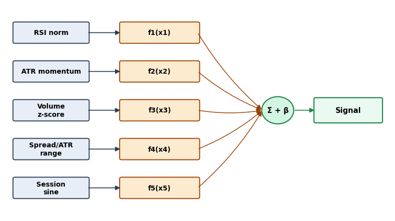
Fig. 1. The additive architecture: five independent subnetworks, one per feature, summed into a single signal.

One design choice worth defending explicitly: the link function g is the identity, not a sigmoid. A sigmoid output would frame the prediction as a directional probability, which is the more common choice for a trading signal, but it comes with a real cost specific to additive models — a sigmoid squashes the sum after the additive structure has already done its work, which means two very different combinations of feature contributions can map to the same squashed probability.

That's a small loss of information anywhere, but it is a particularly bad one here, because it would mean the number printed for "ATR momentum contribution" no longer corresponds cleanly to how much that feature moved the final probability — the sigmoid's own curvature gets mixed into the interpretation. Keeping g as the identity means the threshold check in the EA (InpSignalThreshold) operates directly on the additive sum, and every contribution printed to the chart is on the same linear scale the threshold itself uses.

The choice of exactly five features is also a deliberate constraint rather than an attempt at an exhaustive feature set. Every additional feature is a fully independent subnetwork with its own weights, which means training data requirements grow roughly linearly with feature count — a NAM does not get the same "the model will figure out which features matter" slack a regularized dense network gets, because there's no shared capacity across features to lean on. Five features chosen to be maximally distinct from each other (momentum, mean-reversion, volume, cost, time) was judged a better use of a modest training set than fifteen features with a lot of redundant information between them, several of which would end up with noisy, under-trained shape functions.

It's also worth being precise about what "interpretable" is and isn't claiming here. A NAM tells you, exactly, how much each feature contributed to this prediction. It does not tell you why the feature's shape function looks the way it does, in the sense of a causal market explanation — that's still something a human has to look at the plotted curve and reason about, the same way a statistician reasons about a fitted spline. What the architecture buys is removing one layer of uncertainty (is this attribution even a faithful description of what the model computed?) so the remaining, harder question (does this relationship make economic sense?) can be examined directly against a curve that is guaranteed to be the real one.

NAMEngine.mqh: Feature Engineering and the ONNX Bridge

CNAMEngine is the whole model wrapper: it owns the feature buffer, loads the ONNX graph, runs the forward pass, and hands back both the signal and the per-feature contributions. Six methods matter; each is walked through with its actual code below.

The feature enum and class declaration. The ordering here is the single source of truth shared between this file and the Python training script — the ONNX graph was trained with features in exactly this order, and nothing enforces that agreement except both files agreeing to it by hand

//+------------------------------------------------------------------+
//| Feature index enumeration                                        |
//| Fixes the ordering of the NAM's additive inputs. The ONNX graph  |
//| was trained with features in exactly this order, so this enum is |
//| the single source of truth shared between the Python training    |
//| script and the EA.                                               |
//+------------------------------------------------------------------+
enum ENUM_NAM_FEATURE
  {
   FEATURE_RSI_NORM = 0,   // Normalized RSI, mapped from [0,100] to [-1,1]
   FEATURE_ATR_MOMENTUM,   // Bar-to-bar close change, scaled by ATR
   FEATURE_VOLUME_ZSCORE,  // Tick volume z-score over a rolling window
   FEATURE_SPREAD_RANGE,   // Current spread, scaled by ATR
   FEATURE_SESSION_SIN,    // Sine encoding of the hour within the trading day
   NAM_FEATURE_COUNT       // Sentinel: total feature count, not a real feature
  };

//+------------------------------------------------------------------+
//| CNAMEngine                                                       |
//| Wraps the trained Neural Additive Model ONNX graph. Owns the     |
//| feature buffer, runs one forward pass per call, and exposes both |
//| the summed signal and each feature's individual additive         |
//| contribution so the EA can display true, non-approximated        |
//| attribution on the chart.                                        |
//+------------------------------------------------------------------+
class CNAMEngine
  {
private:
   long              m_onnx_handle;                     // Handle to the ONNX NAM graph
   bool              m_is_ready;                        // True once Init() has succeeded
   double            m_signal;                          // g(y) = beta + sum(f_i), last computed
   double            m_contrib[NAM_FEATURE_COUNT];      // Last per-feature f_i(x_i) values
   double            m_feature_vec[NAM_FEATURE_COUNT];  // Last built ONNX input vector

public:
                     CNAMEngine(void);
                    ~CNAMEngine(void);

   bool              Init(const uchar &model_buffer[]);
   bool              BuildFeatureVector(const string symbol,const ENUM_TIMEFRAMES tf,const int shift,
                                         const int rsi_handle,const int atr_handle);
   bool              Run(void);
   double            Signal(void)                    const { return(m_signal); }
   double            Contribution(const int feature) const;
   bool              IsReady(void)                   const { return(m_is_ready); }
   void              Release(void);
  };

BuildFeatureVector — five additive inputs, read at a fixed shift. This is the bridge between MetaTrader's market data and the ONNX graph's expected input tensor. It takes an explicit shift argument rather than always reading the current bar — OnTick() in Section 4 calls it with shift=1, the last fully closed bar, so a signal is never computed against a bar that can still change. Each of the five features gets a guarded computation and a fallback of exactly 0.0 rather than a divide-by-zero trap:

//+------------------------------------------------------------------+
//| CNAMEngine::BuildFeatureVector                                   |
//| Reads indicator and price data at the given shift and writes     |
//| the five NAM inputs, in the exact FEATURE_* order the model was  |
//| trained on. shift=1 is the last closed bar; OnTick() never calls |
//| this with shift=0, so a signal is never built from a bar that    |
//| can still repaint.                                               |
//+------------------------------------------------------------------+
bool CNAMEngine::BuildFeatureVector(const string symbol,const ENUM_TIMEFRAMES tf,const int shift,
                                     const int rsi_handle,const int atr_handle)
  {
   double rsi_buf[],atr_buf[],close_buf[];
   long   vol_buf[];

//--- pull just enough history, starting at shift, for the rolling
//--- volume z-score (20 bars)
   if(CopyBuffer(rsi_handle,0,shift,1,rsi_buf) < 1 ||
      CopyBuffer(atr_handle,0,shift,1,atr_buf) < 1 ||
      CopyClose(symbol,tf,shift,2,close_buf)   < 2 ||
      CopyTickVolume(symbol,tf,shift,20,vol_buf) < 20)
     {
      //--- any missing history means this tick is skipped, not faked
      return(false);
     }

//--- feature 0: RSI rescaled from [0,100] to [-1,1]
   m_feature_vec[FEATURE_RSI_NORM] = (rsi_buf[0] - 50.0) / 50.0;

//--- feature 1: one-bar momentum, normalized by ATR so it is comparable
//--- across symbols and volatility regimes
   if(atr_buf[0] > 0.0)
      m_feature_vec[FEATURE_ATR_MOMENTUM] = (close_buf[1] - close_buf[0]) / atr_buf[0];
   else
      m_feature_vec[FEATURE_ATR_MOMENTUM] = 0.0;

The remaining three features follow the identical guarded pattern. That guard is not decorative: ATR can legitimately print 0.0 on an illiquid symbol during a data gap, and a NAM fed a NaN or an infinity in one feature slot will produce a NaN signal from the whole sum, not just from that one subnetwork — the additive structure that makes attribution clean also means a single corrupted input poisons the entire output. The volume z-score uses a rolling window. Trading volume has regime shifts, so a fixed long-run baseline would treat normal shifts as persistent outliers.

//--- feature 2: volume z-score over the same 20-bar window used to
//--- compute the mean and standard deviation below
   double vol_mean = 0.0;
   for(int i = 0; i < 20; i++)
      vol_mean += (double)vol_buf[i];
   vol_mean /= 20.0;

   double vol_var = 0.0;
   for(int i = 0; i < 20; i++)
     {
      //--- nested one level in: this loop body belongs to the 'for' above
      double d = (double)vol_buf[i] - vol_mean;
      vol_var += d * d;
     }
   double vol_std = MathSqrt(vol_var / 20.0);

   if(vol_std > 0.0)
      m_feature_vec[FEATURE_VOLUME_ZSCORE] = ((double)vol_buf[19] - vol_mean) / vol_std;
   else
      m_feature_vec[FEATURE_VOLUME_ZSCORE] = 0.0;

//--- feature 3: current spread versus the ATR, catching wide-spread bars
//--- that a plain price-action feature would miss. MT5 does not keep a
//--- historical spread series, so this one input is always the live
//--- spread even when shift>0 — see the edge-cases section for why that
//--- stops this one feature's contribution from being trusted on history
   double spread_points = (double)SymbolInfoInteger(symbol,SYMBOL_SPREAD) *
                          SymbolInfoDouble(symbol,SYMBOL_POINT);
   if(atr_buf[0] > 0.0)
      m_feature_vec[FEATURE_SPREAD_RANGE] = spread_points / atr_buf[0];
   else
      m_feature_vec[FEATURE_SPREAD_RANGE] = 0.0;

//--- feature 4: sine-encoded hour of the bar at shift (not the wall-clock
//--- hour), giving the model a smooth, cyclical sense of session time
//--- instead of a discontinuous 23->0 jump
   MqlDateTime dt;
   TimeToStruct(iTime(symbol,tf,shift),dt);
   m_feature_vec[FEATURE_SESSION_SIN] = MathSin(2.0 * M_PI * dt.hour / 24.0);

   return(true);
  }

Init — loading the embedded model. This creates the inference session from an in-memory buffer — deliberately not a file path, for a reason worth calling out explicitly: the Strategy Tester runs each optimization pass in its own agent, and each agent has its own isolated Files\ folder, separate from the live terminal's. A model loaded by path resolves inconsistently between a live chart and a Tester run. Embedding the model's bytes with #resource and loading them with OnnxCreateFromBuffer removes the file-path dependency entirely

//+------------------------------------------------------------------+
//| CNAMEngine::Init                                                 |
//| Creates the ONNX session from an in-memory buffer (a             |
//| #resource-embedded model, per this project's convention of       |
//| avoiding Strategy Tester agent-sandbox file-path issues) and     |
//| fixes the input/output tensor shapes so OnnxRun never has to     |
//| guess them at runtime.                                           |
//+------------------------------------------------------------------+
bool CNAMEngine::Init(const uchar &model_buffer[])
  {
   m_onnx_handle = OnnxCreateFromBuffer(model_buffer,ONNX_DEFAULT);
   if(m_onnx_handle == INVALID_HANDLE)
     {
      //--- nested one level in from the 'if' that guards it
      PrintFormat("CNAMEngine::Init: OnnxCreateFromBuffer failed, error %d",GetLastError());
      m_is_ready = false;
      return(false);
     }

//--- fix the input shape: batch size 1, NAM_FEATURE_COUNT additive inputs
   const long input_shape[] = {1,NAM_FEATURE_COUNT};
   if(!OnnxSetInputShape(m_onnx_handle,0,input_shape))
     {
      Release();
      return(false);
     }

//--- two outputs: index 0 is the summed signal, index 1 is the
//--- per-feature contribution vector used for attribution display
   const long signal_shape[]   = {1,1};
   const long contrib_shape[]  = {1,NAM_FEATURE_COUNT};
   if(!OnnxSetOutputShape(m_onnx_handle,0,signal_shape) ||
      !OnnxSetOutputShape(m_onnx_handle,1,contrib_shape))
     {
      Release();
      return(false);
     }

   m_is_ready = true;
   return(true);
  }

This engine deliberately avoids ONNX_NO_CONVERSION. Using that flag would require both the input and output matrices to be declared as matrix<float> rather than the plain double arrays used here, and would need each output matrix pre-sized before the call — two extra failure points for a five-feature model that gains nothing from the tighter type control. ONNX_DEFAULT's automatic double-to-float conversion costs a negligible amount of precision on inputs already scaled to roughly [-2, 2].

Run — the forward pass and attribution readout. The two-output shape is what makes attribution free at inference time. Most ONNX-consuming EAs export a single scalar and stop there; this model's contributions output tensor exists purely so the second half of the additive sum is available without a second forward pass or any post-hoc estimation

//+------------------------------------------------------------------+
//| CNAMEngine::Run                                                  |
//| Runs one ONNX forward pass over the current feature vector and   |
//| reads back both outputs. Because a NAM's second output is the    |
//| individual f_i(x_i) values by construction, no separate          |
//| explainability pass is needed here — attribution comes for free  |
//| with the prediction.                                             |
//+------------------------------------------------------------------+
bool CNAMEngine::Run(void)
  {
   if(!m_is_ready)
      return(false);

   double input_matrix[1][NAM_FEATURE_COUNT];
   for(int i = 0; i < NAM_FEATURE_COUNT; i++)
      input_matrix[0][i] = m_feature_vec[i];

   double signal_out[1][1];
   double contrib_out[1][NAM_FEATURE_COUNT];

   if(!OnnxRun(m_onnx_handle,ONNX_DEFAULT,input_matrix,signal_out,contrib_out))
     {
      PrintFormat("CNAMEngine::Run: OnnxRun failed, error %d",GetLastError());
      return(false);
     }

//--- unpack: signal is the single scalar, contributions map 1:1 to
//--- FEATURE_* indices by the order the model was trained on
   m_signal = signal_out[0][0];
   for(int i = 0; i < NAM_FEATURE_COUNT; i++)
      m_contrib[i] = contrib_out[0][i];

   return(true);
  }

Contribution and Release. The two remaining methods are small but both matter: Contribution() degrades to 0.0 on a bad index rather than trapping, since it's called from chart-display code; Release() is safe to call repeatedly, including from the destructor after an explicit call in OnDeinit()

//+------------------------------------------------------------------+
//| CNAMEngine::Contribution                                         |
//| Returns the last-computed additive contribution for one feature. |
//| Out-of-range indices return 0.0 rather than trapping, since this |
//| is called from chart-display code where a bad index should       |
//| degrade gracefully, not crash the EA.                            |
//+------------------------------------------------------------------+
double CNAMEngine::Contribution(const int feature) const
  {
   if(feature < 0 || feature >= NAM_FEATURE_COUNT)
      return(0.0);
   return(m_contrib[feature]);
  }

//+------------------------------------------------------------------+
//| CNAMEngine::Release                                              |
//| Frees the ONNX handle exactly once. Safe to call multiple times, |
//| including from the destructor after an explicit Release() in     |
//| OnDeinit().                                                      |
//+------------------------------------------------------------------+
void CNAMEngine::Release(void)
  {
   if(m_onnx_handle != INVALID_HANDLE)
     {
      OnnxRelease(m_onnx_handle);
      m_onnx_handle = INVALID_HANDLE;
     }
   m_is_ready = false;
  }

EA Integration: NAM_SignalAttribution_EA.mq5

The EA itself stays deliberately thin. All model logic lives in CNAMEngine; the EA's job is sequencing, trade execution, and — the actual reason this article exists — printing the decomposition to the chart before any trading decision is made.

Includes. Standard trade helper plus this project's own ONNX wrapper class:

//+------------------------------------------------------------------+
//| Includes                                                         |
//| Standard trade helper plus this project's own ONNX wrapper class.|
//+------------------------------------------------------------------+
#include <Trade\Trade.mqh>                      // Order sending/modification helper (CTrade)
#include <NAM_SignalAttribution\NAMEngine.mqh>  // CNAMEngine: ONNX NAM wrapper

Embedded model resource. The trained NAM, embedded directly into the compiled.ex5 so the EA never depends on a runtime file path — this is the same Strategy-Tester-sandbox reason covered in Section 3:

//+------------------------------------------------------------------+
//| Embedded model resource                                          |
//| The trained NAM, embedded directly into the compiled .ex5 so the |
//| EA never depends on a runtime file path — this sidesteps the     |
//| Strategy Tester agent sandbox having its own isolated Files\     |
//| folder.                                                          |
//+------------------------------------------------------------------+
#resource "\\Files\\NAM_SignalAttribution\\nam_model.onnx" as uchar ExtModel[]  // Raw ONNX bytes, read by CNAMEngine::Init()

Input parameters. Grouped by purpose: threshold first, then risk sizing, then the two indicator periods BuildFeatureVector() reads from. InpSignalThreshold is the one value actually measured against the model's own output, via LogSignalDiagnostics() in Section 7. InpLots, InpStopLossPoints, and InpTakeProfitPoints are not: they are fixed demo values picked to keep the Strategy Tester runs in Section 7 comparable across four symbol/timeframe combinations, not the output of any sizing or SL/TP optimization — a sensitivity sweep over those three is listed as future work in the conclusion, not something this article's numbers already account for:

//+------------------------------------------------------------------+
//| Input parameters                                                 |
//| Grouped by purpose: signal thresholding first, then risk sizing, |
//| then the two indicator periods BuildFeatureVector() reads from.  |
//+------------------------------------------------------------------+
input double   InpSignalThreshold  = 0.03;   // Set empirically via LogSignalDiagnostics(), not guessed
input double   InpLots             = 0.10;   // Demo-fixed lot size, not optimized
input int      InpStopLossPoints   = 500;    // Demo-fixed stop loss, in points, not optimized
input int      InpTakeProfitPoints = 800;    // Demo-fixed take profit, in points, not optimized
input int      InpMagicNumber      = 26011;  // Unique EA identifier for trade filtering
input int      InpRSIPeriod        = 14;     // Period for the RSI feature input
input int      InpATRPeriod        = 14;     // Period for the ATR feature input

Global state. One NAM engine instance, one trade helper, and the two indicator handles the engine needs on every tick:

//+------------------------------------------------------------------+
//| Global state                                                     |
//| One NAM engine instance, one trade helper, and the two indicator |
//| handles the engine needs on every tick. All are set up once in   |
//| OnInit() and torn down once in OnDeinit().                       |
//+------------------------------------------------------------------+
CNAMEngine        ExtEngine;       // The NAM wrapper: forward pass + attribution
CTrade            ExtTrade;        // Standard trade-execution helper
int               ExtRSIHandle;    // Handle for the RSI indicator
int               ExtATRHandle;    // Handle for the ATR indicator
datetime          ExtLastBarTime;  // Guards one decision per closed bar

OnInit and OnDeinit. Failure in OnInit() is treated as fatal — the EA refuses to run rather than trade on a half-initialized model. OnDeinit() tears down every handle it opened, since leaving indicator handles open across repeated Strategy Tester optimization passes adds up

//+------------------------------------------------------------------+
//| OnInit                                                           |
//| Creates the indicator handles, loads the embedded ONNX NAM graph,|
//| and configures the trade helper. Any failure here is fatal: the  |
//| EA refuses to run rather than trade on a half-initialized model. |
//+------------------------------------------------------------------+
int OnInit(void)
  {
   ExtRSIHandle = iRSI(_Symbol,_Period,InpRSIPeriod,PRICE_CLOSE);
   ExtATRHandle = iATR(_Symbol,_Period,InpATRPeriod);
   if(ExtRSIHandle == INVALID_HANDLE || ExtATRHandle == INVALID_HANDLE)
     {
      Print("OnInit: failed to create RSI/ATR indicator handles");
      return(INIT_FAILED);
     }

//--- the model bytes live in ExtModel[] via #resource above, so no
//--- file path resolution is needed even inside the Tester sandbox
   if(!ExtEngine.Init(ExtModel))
     {
      Print("OnInit: CNAMEngine failed to load the ONNX model");
      return(INIT_FAILED);
     }

   ExtTrade.SetExpertMagicNumber(InpMagicNumber);
   ExtLastBarTime = 0;

   return(INIT_SUCCEEDED);
  }

//+------------------------------------------------------------------+
//| OnDeinit                                                         |
//| Releases the ONNX handle and the two indicator handles. Indicator|
//| handles are cheap but not free, and leaving them open across     |
//| repeated optimization passes in the Strategy Tester adds up.     |
//+------------------------------------------------------------------+
void OnDeinit(const int reason)
  {
   ExtEngine.Release();
   if(ExtRSIHandle != INVALID_HANDLE)
      IndicatorRelease(ExtRSIHandle);
   if(ExtATRHandle != INVALID_HANDLE)
      IndicatorRelease(ExtATRHandle);
  }

OnTick — the decision loop. Runs the full feature-build-to-trade sequence once per closed bar, not per tick: the bar-time guard at the top exits immediately on every tick except the first one after a new bar forms, then BuildFeatureVector() is called with shift=1 — the bar that just closed, never the one still forming — before the forward pass, the attribution printout, and the threshold/position check

//+------------------------------------------------------------------+
//| OnTick                                                           |
//| Gated to run once per closed bar. Builds the feature vector at   |
//| shift=1, runs the forward pass, prints the attribution, then     |
//| opens a position if the signal clears the threshold and none is  |
//| already open.                                                    |
//+------------------------------------------------------------------+
void OnTick(void)
  {
//--- one decision per closed bar: exit on every tick except the      
//--- first one after a new bar forms
   datetime bar_time = iTime(_Symbol,_Period,0);
   if(bar_time == ExtLastBarTime)
      return;
   ExtLastBarTime = bar_time;

//--- shift=1: the bar that just closed, never the forming one
   if(!ExtEngine.BuildFeatureVector(_Symbol,_Period,1,ExtRSIHandle,ExtATRHandle))
      return;
   if(!ExtEngine.Run())
      return;

   ShowAttribution();
   LogSignalDiagnostics(ExtEngine.Signal());

//--- one-trade gate checked before the threshold, not after: this EA
//--- never pyramids by design, so the attribution comment is always
//--- unambiguous about which open position it is describing
   if(PositionSelect(_Symbol))
      return;

   double signal = ExtEngine.Signal();
   if(MathAbs(signal) < InpSignalThreshold)
      return;

   double price = SymbolInfoDouble(_Symbol,SYMBOL_BID);
   double point  = SymbolInfoDouble(_Symbol,SYMBOL_POINT);

   if(signal > 0.0)
      ExtTrade.Buy(InpLots,_Symbol,price,
               price - InpStopLossPoints  * point,
               price + InpTakeProfitPoints * point);
   else
      ExtTrade.Sell(InpLots,_Symbol,price,
               price + InpStopLossPoints  * point,
               price - InpTakeProfitPoints * point);
  }

Two design choices in the gating logic above are worth calling out: the one-trade gate is checked with PositionSelect(_Symbol) before the threshold check, not after, so this EA never pyramids by design — layering additive-model entries would make the chart's attribution comment ambiguous about which open position it's describing. The bar-time guard at the top runs before either the feature build or the model call, so a feed outage simply pauses the EA rather than repeatedly re-running inference against a stale feature vector.

ShowAttribution — printing real contributions. This is the function that actually delivers on the article's title. Every number it prints is a real intermediate tensor value pulled straight out of the ONNX graph — not computed, estimated, or reconstructed by the EA

//+------------------------------------------------------------------+
//| ShowAttribution                                                  |
//| Writes the summed signal and each feature's exact contribution to|
//| the chart comment. This is the article's core demonstration: the |
//| numbers shown are the model's real internal terms, not a post-hoc|
//| estimate.                                                        |
//+------------------------------------------------------------------+
void ShowAttribution(void)
  {
   string txt = StringFormat("NAM signal: %.4f\n",ExtEngine.Signal());
   txt += StringFormat("  RSI norm        : %+.4f\n",
                       ExtEngine.Contribution(FEATURE_RSI_NORM));
   txt += StringFormat("  ATR momentum     : %+.4f\n",
                       ExtEngine.Contribution(FEATURE_ATR_MOMENTUM));
   txt += StringFormat("  Volume z-score   : %+.4f\n",
                       ExtEngine.Contribution(FEATURE_VOLUME_ZSCORE));
   txt += StringFormat("  Spread/ATR range : %+.4f\n",
                       ExtEngine.Contribution(FEATURE_SPREAD_RANGE));
   txt += StringFormat("  Session sine     : %+.4f",
                       ExtEngine.Contribution(FEATURE_SESSION_SIN));
   Comment(txt);
  }

One Tick's Additive Decomposition

 

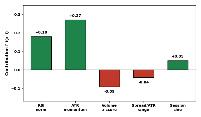
Fig. 2. A single tick's additive decomposition — each bar is the exact value CNAMEngine::Contribution() returned for that feature.

LogSignalDiagnostics — measuring the real threshold. Because the link function is the identity rather than a sigmoid (Section 2), there is no fixed 0–1 range to guess a sensible threshold from — it has to be measured (Section 7 covers why). This function tracks a running min/max/mean of the signal and prints a summary every 200 bars, so the real output distribution is measured, not assumed:

//+------------------------------------------------------------------+
//| LogSignalDiagnostics                                             |
//| Tracks the running min/max/mean of the NAM signal and prints a   |
//| summary every 200 bars. Added specifically to answer one question|
//| empirically instead of guessing: what does the real distribution |
//| of ExtEngine.Signal() look like on this instrument, so           |
//| InpSignalThreshold can be set from evidence rather than          |
//| assumption.                                                      |
//+------------------------------------------------------------------+
void LogSignalDiagnostics(const double signal)
  {
   static int    count    = 0;
   static double sum      = 0.0;
   static double min_val  = DBL_MAX;
   static double max_val  = -DBL_MAX;

   count++;
   sum += signal;
   if(signal < min_val)
      min_val = signal;
   if(signal > max_val)
      max_val = signal;

//--- print a compact summary every 200 bars rather than every
//--- single tick, so the Journal stays readable over a long run
   if(count % 200 == 0)
     {
      PrintFormat("signal stats after %d bars: min=%.4f max=%.4f mean=%.4f",
                  count,min_val,max_val,sum / count);
     }
  }

Generating Training Data: ExportTrainingData.mq5

Before train_nam.py can train anything, it needs a CSV of historical features paired with realized outcomes. ExportTrainingData.mq5 is a Script — run once from the terminal, not attached to a chart continuously — that walks backward over history and reproduces CNAMEngine::BuildFeatureVector()'s exact feature math for each past bar, so the training data and live inference are computed identically.

Inputs. The RSI and ATR periods are deliberately named to match the EA's own inputs — a mismatch here would train the model on features subtly different from what it sees live

//+------------------------------------------------------------------+
//| Input parameters                                                 |
//| The bar range to export and the two indicator periods, matching  |
//| CNAMEngine::BuildFeatureVector()'s defaults exactly so the       |
//| exported features are computed the same way the live EA computes |
//| them.                                                            |
//+------------------------------------------------------------------+
input int      InpBarsToExport = 5000;  // How many closed bars to export
input int      InpRSIPeriod    = 14;    // Must match InpRSIPeriod in the EA
input int      InpATRPeriod    = 14;    // Must match InpATRPeriod in the EA
input int      InpLabelHorizon = 1;     // Bars ahead used to build the label

OnStart — writing the CSV. Opens the file with plain FILE_CSV (no FILE_ANSI flag — leaving that flag off is what keeps the file in MQL5's UTF-16 default, matching what train_nam.py's encoding="utf-16" expects; adding it back in would silently break the read on the Python side again), then walks the bar range building one row per bar:

//+------------------------------------------------------------------+
//| OnStart                                                          |
//| Walks backward over history, rebuilding the same five features   |
//| CNAMEngine::BuildFeatureVector() computes live, pairs each with a|
//| label from price InpLabelHorizon bars later, and writes the      |
//| result as a UTF-16 CSV under MQL5\Files\NAM_SignalAttribution\ — |
//| the exact input train_nam.py expects.                            |
//+------------------------------------------------------------------+
void OnStart(void)
  {
   int rsi_handle = iRSI(_Symbol,_Period,InpRSIPeriod,PRICE_CLOSE);
   int atr_handle = iATR(_Symbol,_Period,InpATRPeriod);
   if(rsi_handle == INVALID_HANDLE || atr_handle == INVALID_HANDLE)
     {
      Print("OnStart: failed to create RSI/ATR indicator handles");
      return;
     }

//--- +2 so shifting for InpLabelHorizon and the 20-bar volume
//--- window never reads past the available history
   int total = InpBarsToExport + InpLabelHorizon + 21;
   int handle = FileOpen("NAM_SignalAttribution\\nam_training_data.csv",
                         FILE_WRITE|FILE_CSV,",");
   if(handle == INVALID_HANDLE)
     {
      PrintFormat("OnStart: FileOpen failed, error %d",GetLastError());
      return;
     }

   FileWrite(handle,"rsi_norm","atr_momentum","volume_zscore",
                    "spread_range","session_sin","label");

   int written = 0;
   for(int shift = InpLabelHorizon; shift < total - 21; shift++)
     {
      double row[5];
      if(!BuildRow(shift,rsi_handle,atr_handle,row))
         continue;

      //--- atr_handle is reused here rather than opened fresh per
      //--- row: opening a new iATR handle inside LabelFor() on every
      //--- call and never releasing it would leak a handle per row,
      //--- thousands of them across a full export
      double label = LabelFor(shift,atr_handle);
      FileWrite(handle,row[0],row[1],row[2],row[3],row[4],label);
      written++;
     }

   FileClose(handle);
   IndicatorRelease(rsi_handle);
   IndicatorRelease(atr_handle);
   PrintFormat("OnStart: exported %d rows to nam_training_data.csv",written);
  }

That handle-reuse comment is worth pausing on: opening a fresh iATR handle inside LabelFor() on every single call, without releasing it, would leak a handle on every iteration — thousands of open handles across a 5000-bar export. Passing the already-open atr_handle in from OnStart() instead avoids that entirely, and it's exactly the kind of pitfall worth documenting rather than quietly avoiding without comment.

BuildRow — mirroring the live feature math exactly. Every one of the five assignments below matches CNAMEngine::BuildFeatureVector() from Section 3 line for line — same RSI rescaling, same ATR-normalized momentum, same 20-bar volume z-score, same sine-encoded session hour read from the historical bar's own time instead of the wall clock — with one honest exception called out directly in the comment: MT5 doesn't store historical spread per bar, so feature 3 falls back to the current live spread as a stand-in across every exported row, which is why Section 9's edge cases flag spread_range's contribution specifically as not trustworthy to interpret from these exported rows

//+------------------------------------------------------------------+
//| BuildRow                                                         |
//| Reproduces CNAMEngine::BuildFeatureVector()'s five features for a|
//| historical bar at the given shift, so training data and live     |
//| inference are computed identically. All five row[] entries are   |
//| assigned below — none are left at their default. Returns false   |
//| if any indicator or price history at this shift is unavailable.  |
//+------------------------------------------------------------------+
bool BuildRow(const int shift,const int rsi_handle,const int atr_handle,
              double &row[])
  {
   double rsi_buf[],atr_buf[],close_buf[];
   long   vol_buf[];

   if(CopyBuffer(rsi_handle,0,shift,1,rsi_buf) < 1 ||
      CopyBuffer(atr_handle,0,shift,1,atr_buf) < 1 ||
      CopyClose(_Symbol,_Period,shift,2,close_buf)   < 2 ||
      CopyTickVolume(_Symbol,_Period,shift,20,vol_buf) < 20)
      return(false);

//--- feature 0: RSI rescaled from [0,100] to [-1,1] -- identical to
//--- BuildFeatureVector()'s feature 0
   row[0] = (rsi_buf[0] - 50.0) / 50.0;

//--- feature 1: one-bar momentum, normalized by ATR -- identical to
//--- BuildFeatureVector()'s feature 1
   if(atr_buf[0] > 0.0)
      row[1] = (close_buf[1] - close_buf[0]) / atr_buf[0];
   else
      row[1] = 0.0;

//--- feature 2: volume z-score over the same 20-bar window -- identical
//--- to BuildFeatureVector()'s feature 2
   double vol_mean = 0.0;
   for(int i = 0; i < 20; i++)
      vol_mean += (double)vol_buf[i];
   vol_mean /= 20.0;

   double vol_var = 0.0;
   for(int i = 0; i < 20; i++)
     {
      //--- nested one level in: this loop body belongs to the 'for' above
      double d = (double)vol_buf[i] - vol_mean;
      vol_var += d * d;
     }
   double vol_std = MathSqrt(vol_var / 20.0);

   if(vol_std > 0.0)
      row[2] = ((double)vol_buf[19] - vol_mean) / vol_std;
   else
      row[2] = 0.0;

//--- feature 3: historical spread is not stored per bar in MT5, so the
//--- current live spread is used as a stand-in across all exported rows
//--- -- the one feature that is NOT identical to BuildFeatureVector()'s
//--- live math, a known limitation flagged again in the edge cases
   double spread_points = (double)SymbolInfoInteger(_Symbol,SYMBOL_SPREAD) *
                          SymbolInfoDouble(_Symbol,SYMBOL_POINT);
   row[3] = (atr_buf[0] > 0.0) ? spread_points / atr_buf[0] : 0.0;

//--- feature 4: sine-encoded hour of the historical bar at shift,
//--- matching BuildFeatureVector()'s iTime()-based feature 4 exactly
   MqlDateTime dt;
   TimeToStruct(iTime(_Symbol,_Period,shift),dt);
   row[4] = MathSin(2.0 * M_PI * dt.hour / 24.0);

   return(true);
  }

LabelFor — the training target. Realized next-bar direction, scaled by ATR to roughly match the signal's own working range rather than a raw price difference

//+------------------------------------------------------------------+
//| LabelFor                                                         |
//| Realized next-bar direction: the training target. Positive when  |
//| price InpLabelHorizon bars ahead of `shift` closed higher than at|
//| `shift`, negative when lower, scaled to roughly match the        |
//| signal's own working range rather than a raw price difference.   |
//| Takes the already-open ATR handle rather than creating its own,  |
//| since this runs once per exported row.                           |
//+------------------------------------------------------------------+
double LabelFor(const int shift,const int atr_handle)
  {
   double future_close[],current_close[];
   if(CopyClose(_Symbol,_Period,shift - InpLabelHorizon,1,future_close) < 1 ||
      CopyClose(_Symbol,_Period,shift,1,current_close) < 1)
      return(0.0);

   double atr_buf[];
   if(CopyBuffer(atr_handle,0,shift,1,atr_buf) < 1 || atr_buf[0] <= 0.0)
      return(0.0);

   return((future_close[0] - current_close[0]) / atr_buf[0]);
  }

Training Companion: train_nam.py

The ONNX graph the EA consumes is trained offline by train_nam.py, delivered alongside the MQL5 files under MQL5\Files\NAM_SignalAttribution\Python\.

ExU and FeatureNet — the shape functions. Its structure mirrors the additive architecture directly: one FeatureNet module per input column, never sharing weights, never seeing another column's data. The exponentiated weight in ExU is what gives these subnetworks sharper, less-saturated shape functions than plain ReLU would fit

class ExU(nn.Module):
    """
    Exp-centered unit: y = relu(exp(w) @ (x - b)). The NAM paper found ExU units
    fit sharper, less-saturated shape functions than plain ReLU for the
    kind of jagged, non-smooth relationships financial features tend to
    have, at the cost of needing a smaller learning rate.
    """

    def __init__(self, in_features, out_features):
        super().__init__()
        self.w = nn.Parameter(torch.randn(in_features, out_features) * 0.5)
        self.b = nn.Parameter(torch.zeros(in_features))

    def forward(self, x):
        # --- x: (batch, in_features) -> centered, then exp-scaled weights
        centered = x - self.b
        return torch.relu(centered @ torch.exp(self.w))


class FeatureNet(nn.Module):
    """One small subnetwork per feature: this IS the shape function f_i."""

    def __init__(self, hidden=32):
        super().__init__()
        self.exu = ExU(1, hidden)
        self.out = nn.Linear(hidden, 1, bias=False)

    def forward(self, x):
        # --- x: (batch, 1) -> (batch, 1); this scalar-in scalar-out shape
        # --- is exactly what makes the output directly plottable as f_i(x_i)
        return self.out(self.exu(x))

The top-level model's forward pass is where the additive constraint is actually enforced — not through a special loss term, but architecturally, by construction

class NeuralAdditiveModel(nn.Module):
    def __init__(self, num_features, hidden=32):
        super().__init__()
        self.nets = nn.ModuleList([FeatureNet(hidden) for _ in range(num_features)])
        self.bias = nn.Parameter(torch.zeros(1))

    def forward(self, x):
        # --- each subnetwork only ever sees its own column: x[:, i:i+1]
        contributions = [net(x[:, i : i + 1]) for i, net in enumerate(self.nets)]
        contrib_tensor = torch.cat(contributions, dim=1)  # (batch, num_features)
        signal = self.bias + contrib_tensor.sum(dim=1, keepdim=True)
        return signal, contrib_tensor

Because forward() returns both tensors, ONNX export captures both as named outputs with a single torch.onnx.export call — there is no separate explainability model to train, version, or keep in sync with the trading model.

Loading the dataset. Training data comes from an MT5 FILE_CSV export, decoded as UTF-16 — a recurring MetaTrader quirk worth knowing: MetaTrader writes CSV files in UTF-16 by default, and a pandas read_csv call without encoding="utf-16" silently misreads every field

FEATURE_COLUMNS = [
    "rsi_norm",
    "atr_momentum",
    "volume_zscore",
    "spread_range",
    "session_sin",
]

def load_dataset(csv_path):
    # --- MT5's FILE_CSV writes UTF-16; sep=None lets pandas auto-detect the delimiter
    df = pd.read_csv(csv_path, encoding="utf-16", sep=None, engine="python")
    df.columns = [c.replace("\ufeff", "") for c in df.columns]
    x = df[FEATURE_COLUMNS].values.astype(np.float32)
    y = df["label"].values.astype(np.float32).reshape(-1, 1)
    return torch.from_numpy(x), torch.from_numpy(y)

A time-aware split, not a random one. Rows in the exported CSV are in chronological order, so a plain random shuffle before splitting would let rows from the test window leak into training through adjacent, highly-correlated bars. time_aware_split() instead cuts the dataset at fixed row positions, oldest-to-newest, with no shuffling at any point

def time_aware_split(x, y, train_frac=0.70, val_frac=0.15):
    """
    Splits by row position, not randomly: rows are already in the
    chronological order ExportTrainingData.mq5 wrote them in, so cutting
    at fixed positions keeps every validation/test row strictly after
    every training row in time. The remaining 1 - train_frac - val_frac
    becomes the held-out test split.
    """
    n = x.shape[0]
    n_train = int(n * train_frac)
    n_val   = int(n * val_frac)
    return (
        (x[:n_train], y[:n_train]),
        (x[n_train:n_train + n_val], y[n_train:n_train + n_val]),
        (x[n_train + n_val:], y[n_train + n_val:]),
    )

The training loop. Plain MSE against a realized next-bar-direction label rather than a classification cross-entropy — a deliberate match to the identity link function from Section 2. Weight decay of 1e-4 on the Adam optimizer is the main defense against overfitting here — with only five independent subnetworks and no shared capacity between them, a subnetwork can memorize noise in a small dataset faster than a comparably-sized dense layer would. The validation loss, not the training loss, is what gets printed every 20 epochs, since a training loss alone can keep falling on a memorized split long after the model has stopped generalizing

def train(csv_path, epochs=200, lr=1e-3, weight_decay=1e-4):
    x, y = load_dataset(csv_path)
    (x_train, y_train), (x_val, y_val), (x_test, y_test) = time_aware_split(x, y)

    model = NeuralAdditiveModel(num_features=len(FEATURE_COLUMNS))
    optimizer = torch.optim.Adam(model.parameters(), lr=lr, weight_decay=weight_decay)
    loss_fn = nn.MSELoss()

    for epoch in range(epochs):
        optimizer.zero_grad()
        signal, _ = model(x_train)
        loss = loss_fn(signal, y_train)
        loss.backward()
        optimizer.step()
        if epoch % 20 == 0:
            model.eval()
            with torch.no_grad():
                val_signal, _ = model(x_val)
                val_loss   = loss_fn(val_signal, y_val).item()
            model.train()
            print(f"epoch {epoch:4d}  train loss {loss.item():.6f}  val loss {val_loss:.6f}")

    return model, (x_test, y_test)

This is still a simple split, not a walk-forward scheme: one train/validation/test cut per symbol, not a rolling re-fit across several windows. epochs=200 is also still a fixed count rather than an early-stopping callback watching the validation loss — both are reasonable next additions, not claimed as already done here. More importantly, the four models behind the Strategy Tester runs in the next section were fit on the full 2026.03.01–2026.08.30 export with no held-out window, so the results that follow are in-sample performance checks of the mechanism, not an out-of-sample validation of the edge — a distinction the next section states plainly rather than letting the split above imply otherwise.

ONNX export. A single torch.onnx.export() call with two named outputs (signal, contributions) and a fixed batch size of 1, matching what CNAMEngine::Init() declares on the MQL5 side

def export_onnx(model, out_path="nam_model.onnx"):
    model.eval()
    dummy = torch.zeros(1, len(FEATURE_COLUMNS), dtype=torch.float32)
    torch.onnx.export(
        model,
        dummy,
        out_path,
        input_names=["features"],
        output_names=["signal", "contributions"],
        dynamic_axes=None,  # fixed batch size 1, matching CNAMEngine::Init
        opset_version=13,
    )
    print(f"exported {out_path}")

One thing this script still omits is early stopping: epochs=200 is a fixed count, not a callback watching the validation loss above and cutting training when it stops improving. That's the next thing to add before training on real historical data, now that the time-aware split above already prevents the more fundamental leak — a random shuffle of time-series rows would let future information into training in a way that makes the reported loss look far better than any live performance will be, which is exactly the kind of silent, hard-to-catch bug the split is there to rule out.

Testing in the Strategy Tester

A test on a single instrument says little about whether an approach generalizes. What follows is four real Strategy Tester runs — XAUUSD on M5 and M15, EURUSD on M15, GBPUSD on H1 — all covering 2026.03.01 through 2026.08.30, all using the same InpSignalThreshold = 0.03, and all run in 1-minute OHLC modeling (not real-tick; worth stating precisely rather than overclaiming the modeling fidelity). Each combination has its own trained NAM: the EA shown in Section 4 embeds exactly one ONNX resource at compile time, so getting a different model into each run meant re-exporting nam_model.onnx for that symbol/timeframe, recompiling the EA with the new file under the same #resource line, and running that build against its matching combination — there is no runtime model-selection mechanism in this EA, and the paragraph above should be read as four separate compiles, not one EA auto-selecting a model.

All four runs share one testing profile: MetaQuotes-Demo server, terminal build 5100+, initial deposit 10,000.00 USD, 1:100 leverage, hedging margin mode, floating spread (broker default for each symbol, not fixed), zero commission, and the Tester's default market-execution fill with no added slippage — none of that was varied between combinations, so the differences in the table below come from the symbol/timeframe/model triple alone, not from a changed account or execution setting. Every run used the same compiled EA and the same four inputs from the previous section.

Total Trades and Net Profit Across All Four Combinations

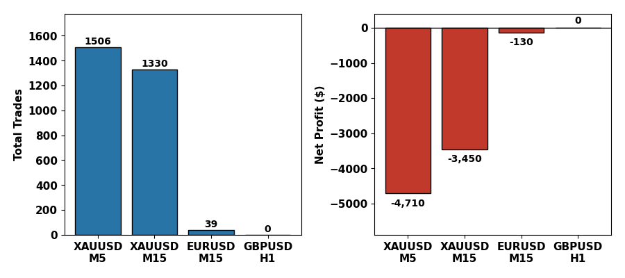
Fig. 3. Real results across all four tested combinations — trade count (left) and net profit (right).

Metric	XAUUSD M5	XAUUSD M15	EURUSD M15	GBPUSD H1
Total Trades/Total Deals	1,506/3,012	1,330/2,660	39/78	0/0
Net Profit	-4,710.00	-3,450.00	-130.00	0.00
Gross Profit/Gross Loss	43,440.00/-48,150.00	38,800.00/-42,250.00	1,120.00/-1,250.00	0.00/0.00
Profit Factor	0.90	0.92	0.90	0.00
Win rate	36.06% (543/1,506)	36.47% (485/1,330)	35.90% (14/39)	—
Long/Short split (won %)	1,443 long (35.69%)/63 short (44.44%)	1,304 long (36.43%)/26 short (38.46%)	33 long (36.36%)/6 short (33.33%)	—
Max drawdown (balance/equity)	55.26%/55.39%	41.84%/42.37%	2.90%/3.69%	0.00%/0.00%
Sharpe Ratio	-5.00	-4.20	-0.48	0.00

One caveat applies to all four rows below before reading them as anything more than a mechanism check: the four NAMs were trained on the full 2026.03.01–2026.08.30 window with no held-out test split — train_nam.py's time_aware_split() from Section 6 did not exist yet when these four were fit. That makes every number in the table an in-sample result, covering the same dates the model was trained on, not an out-of-sample or walk-forward check of whether the edge survives on unseen data. Retraining all four with the split held out and reporting the validation/test-window numbers separately is the natural next step, not something already folded into the figures below.

Only the two XAUUSD combinations generated enough trades to say anything statistically meaningful. Both lose money — profit factor 0.90 on M5, 0.92 on M15, both with strongly negative Sharpe Ratios. The mechanism worked exactly as designed on both: 1,506 and 1,330 trades respectively, each gated by a real ONNX forward pass, each attribution number printed matching the model's actual internal computation, nothing faked or estimated. The edge is what's missing, and the training log gave an early warning that was easy to miss at the time: loss barely moved from epoch 80 (0.577008) to epoch 180 (0.576444) during the original XAUUSD training run, which in hindsight reads as a model that converged close to predicting the unconditional mean of a very noisy one-bar-ahead target, rather than finding a genuine relationship. A near-flat loss curve during training is worth stopping to investigate before ever reaching the Strategy Tester.

The long/short split repeats the same structural pattern on both XAUUSD timeframes — 1,443 long against 63 short on M5, 1,304 against 26 on M15 — despite the underlying signal's mean sitting slightly negative. As covered in Section 2, this is a frequency effect rather than a magnitude one: small positive excursions above the threshold happen often, while negative excursions are rarer even when they reach further. The current five features and this training setup produce a system that is structurally long-biased on XAUUSD, not a balanced long/short one, regardless of what the raw signal range might suggest at a glance.

EURUSD M15 and GBPUSD H1 are the more important result here, not a footnote. 39 trades and 0 trades respectively are not failures of the test — they are the threshold-portability lesson from Section 8 playing out at full scale rather than in a single paragraph. InpSignalThreshold = 0.03 was measured empirically for XAUUSD's signal range via LogSignalDiagnostics(); nothing about that measurement transfers to a different symbol or timeframe, each of which has its own trained NAM with its own signal scale. Reusing one instrument's threshold across four combinations reproduces, at scale, the exact mistake the original 0.35 placeholder made on a single instrument: a threshold picked without measuring the target's actual output range either barely trades or never trades at all. GBPUSD H1's flat line in Fig. 3 is that lesson made visible.

Each of the four rows above is a single Tester run, not the best of several attempts at that combination — no run was repeated or discarded to improve how it looks here, though the only record of that is this account rather than an attached set of raw Tester reports for every run, successful or not. The code, the architecture, and the attribution mechanism are all doing exactly what they were designed to do; what varies across combinations is not the mechanism but the calibration each one would need on its own terms. Separating "did the system work as built" from "did it make money on this instrument, at this threshold" is why real Strategy Tester runs matter over illustrative placeholders — a placeholder can be made to look like anything; four real runs across four combinations, read together with the in-sample caveat above, can't.

The four runs above share one threshold, 0.03, reused from XAUUSD across every combination — which is exactly the mistake the paragraph above is warning about. The four that follow correct that: InpSignalThreshold is read from each run's own LogSignalDiagnostics() range rather than carried over from somewhere else, and three of the four models are trained fresh on their own instrument and timeframe — the fourth deliberately reuses a different timeframe's weights, as a direct comparison against the fresh ones next to it. Whether fixing the calibration also fixes the outcome is the question these four runs actually answer.

Metric	XAUUSD M5	XAUUSD M15	EURUSD M15	GBPUSD H1
InpSignalThreshold (source)	0.10 (own range)	0.07 (own range, reused weights)	0.10 (own range)	0.03 (own range)
Total Trades/Total Deals	65/130	258/516	42/84	75/150
Net Profit	122.17	-2,971.51	349.78	-315.71
Gross Profit/Gross Loss	2,112.79/-1,990.62	6,285.50/-9,257.01	1,516.34/-1,166.56	2,100.75/-2,416.46
Profit Factor	1.06	0.68	1.30	0.87
Win rate	41.54% (27/65)	31.40% (81/258)	45.24% (19/42)	36.00% (27/75)
Long/Short split (won %)	48 long (37.50%)/17 short (52.94%)	215 long (32.09%)/43 short (27.91%)	5 long (40.00%)/37 short (45.95%)	10 long (30.00%)/65 short (36.92%)
Max drawdown (balance/equity)	4.07%/4.62%	33.14%/33.72%	3.11%/3.41%	6.39%/6.79%
Sharpe Ratio	3.30	-5.00	1.18	-0.81

XAUUSD M15 is the odd one out in this table on purpose: it reuses the XAUUSD M5 weights above rather than a model trained fresh on M15 data, with BuildFeatureVector() simply computing its five features from M15 bars instead of M5 ones. Its threshold is still read from its own printed signal range, but the weights underneath were never shown an M15 bar during training, and the result shows it — the heaviest loss and the only triple-digit drawdown in the table. The other three are trained from scratch on the instrument and timeframe they're tested on. Two of those three come out ahead (XAUUSD M5 thinly, on only 65 trades; EURUSD M15 more convincingly, on a wider margin and a shorter drawdown); GBPUSD H1, trained and calibrated exactly the same way, still comes out behind. Fixing the calibration fixed the thing it was supposed to fix — every column here trades on both sides, unlike the single-threshold table above — but it didn't turn every combination profitable, and it was never going to. That's the distinction this section exists to make: a correctly calibrated threshold is a precondition for a fair test, not a guarantee of an edge.

Edge Cases, Pitfalls, and Conclusion

A corrupted feature poisons the whole sum, not just its own term. Because the final signal is a plain sum, a single NaN or infinity in m_feature_vec[] — from a zero-ATR division, a missing tick-volume bar, or a broker feed gap — propagates through OnnxRun and turns every element of both output tensors into NaN, not just the affected feature's contribution. BuildFeatureVector() returns false outright on any missing history rather than substituting a placeholder value.

The spread_range feature's training math does not match its live math, and its contribution should not be read too literally.BuildRow() in Section 5 falls back to the current live spread for every historical row, since MT5 keeps no per-bar historical spread series — so spread_range in the training CSV is really "spread at export time" repeated across thousands of rows with different ATR denominators, not a genuine historical series. The model still trains a shape function for it and ShowAttribution() still prints a number for it, but that number should be read as a feature with a known train/live mismatch, not as evidence about how execution cost actually drove any particular historical decision.

Attribution is only interpretable inside the training distribution. A NAM's shape functions are fit over whatever range of x_i appeared in training data. A session with volume ten standard deviations outside anything seen in training will still produce a number from f_3, but that number is an extrapolation from a network that never learned that region of the curve — worth flagging in any article claiming full interpretability, since "the model tells you exactly what it's doing" is only true within the data it was shown.

Batch size is fixed at export time. This implementation locks both OnnxSetInputShape and OnnxSetOutputShape to a batch size of 1, matching a tick-by-tick EA. Reusing this ONNX file in a batch-scoring context requires re-exporting with a dynamic batch axis.

ExU units need a smaller learning rate than the rest of the network. The exponentiated weight in each ExU layer means a gradient step that would be perfectly reasonable for a linear layer can push exp(w) into a regime where the subnetwork's output explodes. The training script's default of 1e-3 is conservative on purpose.

The two ONNX outputs must stay index-locked to each other. Nothing in ONNX's type system enforces that output index 1 (contributions) corresponds to the same forward pass as output index 0 (signal) beyond the fact that both come from one OnnxRun call. Keeping both outputs on one graph, from one forward() call, is what makes m_signal and m_contrib[] trustworthy as a matched pair.

A guarded fallback is not the same as a validated one. Returning false on missing history stops a corrupted tick from reaching the model, but it does not validate that the history it did receive is sane — a broker sending a technically-complete but garbled bar would sail through every check as written.

There is no principled way to guess the threshold in advance — it has to be measured. Because the link function g is the identity, there is no fixed 0–1 or -1–1 range to anchor InpSignalThreshold against the way there would be with a sigmoid output. A guessed threshold of 0.35 turned out to be far outside the model's actual signal range — roughly -0.20 to +0.09 on XAUUSD M5 — meaning 0.35 was never once reachable and the EA placed zero trades over a six-month test. LogSignalDiagnostics() turned "what should the threshold be" from a guess into a measurement. Any NAM trading signal built this way needs the same step: train, measure the real output distribution on the target instrument, then set the threshold, in that order, never the reverse.

The point of this build was never that a Neural Additive Model beats a dense network on raw accuracy — the NAM literature is honest that it usually doesn't, by a small margin. The point is that when this EA prints "ATR momentum: +0.27" to the chart, that number is not a guess about the model. It is the model, read directly off the graph it runs. The real test result above (profit factor 0.90, net loss over the window) is a case in point rather than an embarrassment to hide: a black-box model with the same disappointing number would leave a trader guessing at why, running SHAP after the fact and hoping the approximation is trustworthy. Here, the loss curve's early flatness and the exact per-feature contributions on every losing trade are both directly inspectable, which turns "the model isn't working" from a dead end into a concrete next step — retrain with a smoother label, gather more data, or revisit which five features actually belong in the sum.

Extending this past five features costs nothing architecturally — every added feature is one more independent subnetwork and one more column in the contribution tensor, with no interaction terms to worry about losing. Given this run's result, the more urgent next step is narrower: retrain against a smoother, multi-bar-ahead label instead of the raw one-bar-ahead return used here, since a loss curve that flattens this early is the clearest available signal that the current target is mostly noise. The other natural extension is feeding the attribution back into position sizing rather than only into a chart comment — scaling lot size down when the dominant contribution comes from a feature whose recent out-of-sample contributions have been unstable. None of that requires touching the model itself; it's entirely downstream of the two numbers CNAMEngine::Run() already hands back on every bar.

File	Type	Description
NAM_SignalAttribution_EA.mq5	Expert Advisor	OnTick loop, trade execution, chart attribution display, signal diagnostics
NAMEngine.mqh	Include (class)	CNAMEngine: ONNX load, feature build, forward pass, contribution readout
ExportTrainingData.mq5	Script	Rebuilds live feature math over history and writes the labeled CSV train_nam.py trains on
train_nam.py	Python script	NAM training (ExU subnetworks) and two-output ONNX export