Developing a Replay System — Market simulation (Part 15): Birth of the SIMULATOR (V) - RANDOM WALK
Introduction
In the last few articles in this series, in which we develop a market replay system, we saw how to simulate, or more precisely, how to generate a kind of virtual simulation of a specific symbol. The goal is to get movement as close to real as possible. Although we have made significant progress from a simple system, very similar to the one used in the strategy tester, to a very interesting model, we have not yet been able to create a model that fits any data set. It needs to be dynamic and at the same time stable enough to be able to generate many possible scenarios with minimal programming effort.
Here we will correct the flaw from the article "Developing a Replay System — Market simulation (Part 14): Birth of the SIMULATOR (IV)". Although we have generated the operating RANDOM WALK principle, it is not entirely adequate when working with values from a predefined file or database. Our case is special: the database will always indicate metrics that must be used and followed. Although the RANDOM WALK system that we previously considered and developed can generate movements very similar to those observed in a real market, it is not suitable for use in a movement simulator. This is because it cannot fully cover the range that must be covered in all cases. In very rare cases we will have complete coverage of the entire range, starting from the opening price to the high or low, completely changing direction when reaching one of the limits and going to the other extreme. In the end, almost by magic, it will find and stop at exactly the price that was determined to be the the closing of the bar.
It may seem impossible, but sometimes it happens. But we cannot rely on chance. We need it at the same time to be as random as possible and be within the allowed limits. It also should fulfill its function - complete and comprehensive coverage of all the points of the bar. By thinking this way and analyzing some abstract mathematical concepts, we can generate a relatively attractive form of supervised RANDOM WALK. At least regarding the fact that all points of interest and certain points will be reached.
The idea itself is simple, although quite unusual; I will not go into unnecessary mathematical details so as not to complicate the explanation. However, along with the code, we will consider the concept that will be used so that you too can understand it, and those who understand can even develop slight variations of what I will present.
Understanding the idea and concept
If you've been following this series or articles, you may have noticed that we started by experimenting and trying to create a system that could cover all price points. To do this, we used a technique very similar to that used in the strategy tester. This technique is based on the typical zigzag movement, which is very common and widely known among those who study the market. For those who are not familiar with it or do not know what it is, please see figure 01 showing its schematic representation.
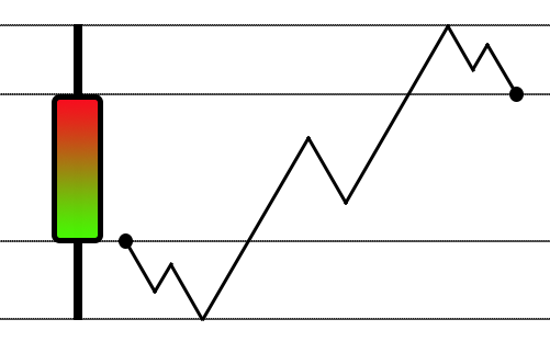
Figure 01 - Typical zigzag movement
Although such modeling is suitable for the strategy tester, it is not always adequate for the replay/simulation system. The reason is simple: the number of orders generated by such a simulation is always significantly less than the actual number, but this does not mean that the model is invalid, just that it is not suitable for use in a system like the one we want to develop. Even if we could find a way for the movement shown in figure 01 to generate a numbre of tickets equivalent to really traded one, the movement itself wouldn't be complex enough. This would simply be an adaptation of the real movement. We need to implement this differently.
We need to find a way that would be as random as possible, but at the same time not complicate the code. Remember: if the complexity of code grows too quickly, it will soon become impossible to maintain and fix. We should always strive to keep things as simple as possible. So you might think that we could simply generate random price values and thus simulate a high enough level of complexity that the movement would be as close to real as possible. However, we cannot afford to accept any price or any number of tickets generated, we must always respect the database. Always.
When you look at the database, you may notice that it contains quite a lot of useful information, in fact, it exists because it is necessary. Figure 02 shows the typical contents of a bars file. Some values that are of real interest are highlighted in it.

Figure 02 - Typical contents of a 1-minute bar file
If we take these values and generate completely random price values, and, I emphasize, keeping within the given range, you get a completely random type of movement. At the same time, this step itself would be far from convenient. Such movement in the real market rarely occurs.
To see what is being generated, let's again convert the things into a graphical format. The result of completely random generation of prices in a given range will look like this:
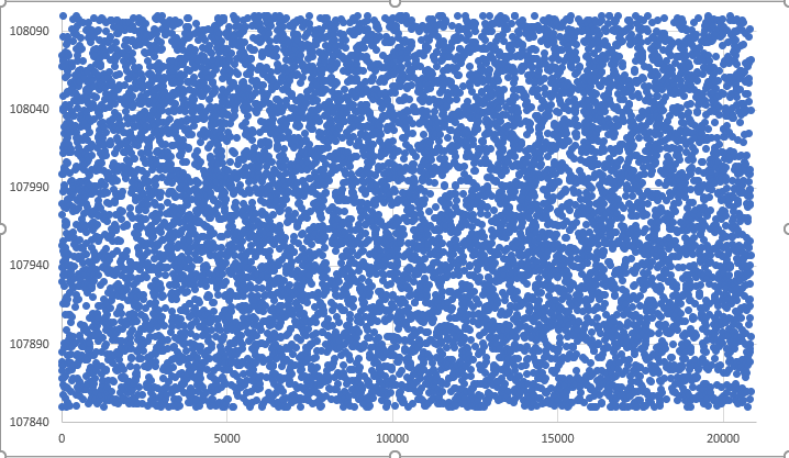
Figure 03 - Graph of the result of totally random values
Such a graph can be obtained using a fairly simple and at the same time very effective method. We've already seen how to do this in Excel, so you can generate a graph like this. This will allow you to more accurately analyze the movement you are creating, based only on the values in the database. Indeed, it is worth learning how to do this, because it enables faster analysis of completely random values. Without this resource, we will feel completely lost in the vast amount of data.
Knowing how to build such graphs, you can more efficiently analyze the situation. And you will understand that the graph presented in Figure 03 is not entirely suitable for our system due to the high degree of randomness present in it. Then we need to look for a way to at least contain this randomness in order to create something more similar to real movement. After a while, you will discover a method that is often used in old video games, where the character seems to move randomly through the game scenario, but in fact everything happens according to fairly simple rules. This method can also be seen in very popular and fun mix-and-match systems such as the Rubik's Cube (Fig. 04), or even in 2D games like 15 Puzzle, in which sliding pieces are used both to solve the problem and to mix up the pieces in the game (Fig. 05).
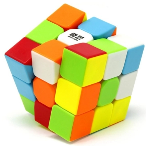
Figure 04 - Rubik's Cube - an example of the RANDOM WALK movement.
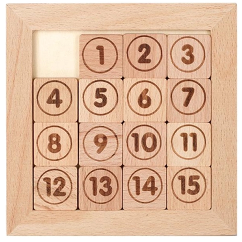
Figure 05 - 15 Puzzle: the simplest RANDOM WALK system
Although at first glance these games do not seem to use RANDOM WALK, they actually do. But not to solve them, although it would be possible to solve them using the RANDOM WALK method, even though it would take much longer than using more suitable methods. To places the pieces in positions that appear to be random, it is necessary to use a formulation involving RANDOM WALK. After that, you try to solve them using a different method, as a child does, returning the parts to the correct place. The same applies to the ticket generation system using RANDOM WALK. In fact, the mathematics behind the RANDOM WALK motion system is essentially the same in all cases, it does not change.
In fact, only the direction system that we will use changes. Try to imagine a completely meaningless movement, but this movement is in 3D space and does not fit into such mathematics. To be honest, teher are very few cases in which this would actually happen. In many of these, the mathematics involved in describing RANDOM WALK can explain the variations that occur over time. Thus, using this mathematics in the "Price x Time" system, we will get a graph similar to the one shown in Fig. 06.
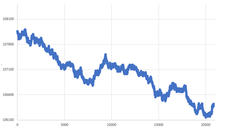
Figure 06 - RANDOM WALK of Price x Time
This kind of thing that follows the same principles as stochastic movements is very similar to the real movement that the market usually shows. However, do not be deceived. The above chart is not of a real asset. It is obtained using a random number generator: one unit is added to or subtracted from the previous price, thus generating a new price. The way we understand whether we are adding or subtracting depends on the rule we are using. You can simply say that any randomly generated ODD number will mean addition, and any EVEN number will mean subtraction. Despite its simplicity, this rule allows you to achieve the desired result. However, the rule can be modified so that any randomly generated number that is a multiple of 5 represents addition, and otherwise subtraction. Simply changing this rule will result in a completely different graph. Even the value that triggers the random generation system changes the situation somewhat.
Although the graph in Fig. 06 is suitable for completely free system, we cannot use it in a simulation system. This is because we must respect the values specified in the database, because this gives us explicit upper and lower bounds for generating the RANDOM WALK. Thus, after making corrections to ensure compliance with these limits, we move from the graph shown in Fig. 06, to the graph shown in Fig. 07.
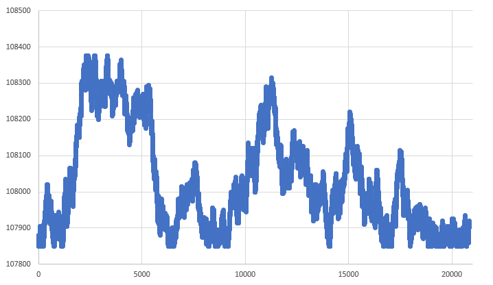
Figure 07 - RANDOM WALK within limits
The system generating the graph shown in Fig. 07 is much more suitable for use in a simulator. Here we have a database that indicates the limits within which we can move. In fact, using equally simple mathematics, we manage to create a system that contains an acceptable level of complexity, and at the same time it is not completely predictable, i.e. we are on the right track. Please note that in the graphs, from the one shown in Fig. 01 to the graph in Fig. 07, the only thing that changed is the level of complexity. Or rather, the randomness present in the last chart is more appropriate. Although the system shown in Fig. 01 is sufficient for the strategy tester, the graph generated and presented in Fig. 07 contains much more things than are needed for the tester. However, for the simulator these things are of paramount importance.
But even with this increase in the level of complexity, observed in graph 07, it is still not quite sufficient for use in the simulator. The only thing we can be sure of when using it is the starting point. In this case we are talking about the OPENING PRICE. It is not possible to guarantee that any of the other points specified in the database (CLOSE, MAXIMUM, MINIMUM) will be affected. And this is a problem, because for the simulator to be truly viable, all the points specified in the database must be touched with absolute certainty.
Based on this, we need to somehow ensure that the graph in Fig. 07 turns into a graph shown in Fig. 08, where we have absolute confidence that these points will actually be reached at a certain point in time.
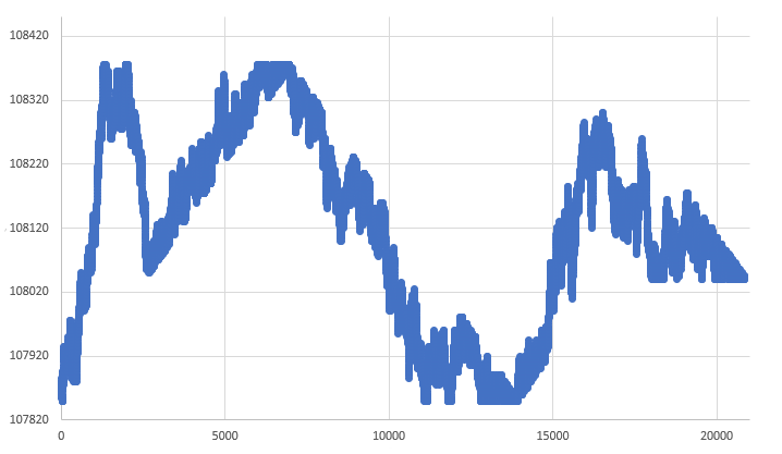
Figure 08 - Forced RANDOM WALK
This type of change involves no more than a few adjustments. But if you look closely at the chart, you can clearly see that the movement is somehow being directed. Even in this case, one cannot help but notice that we have a RANDOM WALK, although not as natural, but still random, as one would expect with stochastic movement. Now I want to draw your attention to the following point: All the graphs discussed above use the same database. It is shown in Fig. 02. However, the best solution is the one shown in Fig. 08, where we actually have a movement that is not as confusing and not as far from the database as in Figure 03. In this case, everything is very similar to what could happen when building a bar.
Based on the concepts shown, I think I've convinced you that the code at the stage described in the previous article is not exactly what we need in the simulator. This is because some points may not have been reached during the period when the random movement occurred. However, instead of forcing these points to appear on the graph, how do you like the idea of making everything more natural?
It is this point that we will consider in the next topic.
Forced RANDOM WALK
Calling it a "forced random walk" does not mean that we will impose a condition on it. However, we will limit the movement in a certain way to make it look as natural as possible while still maintaining its random nature. There is one detail: we will direct the movement to the convergence point. And this is the point you need to visit. So we get a combination between figures 01 and 07, and that's very intriguing, isn't it? But in reality we will not use the path that is usually created as shown in Fig. 01. We take a slightly different approach.
To really understand this, let's look at the random walk code found from the previous article. It is shown below:
inline void Simulation(const MqlRates &rate, MqlTick &tick[])
                        {
#define macroRandomLimits(A, B) (int)(MathMin(A, B) + (((rand() & 32767) / 32767.0) * MathAbs(B - A)))

                                long    il0, max;
                                double  v0, v1;
                                bool    bLowOk, bHighOk;

                                ArrayResize(m_Ticks.Rate, (m_Ticks.nRate > 0 ? m_Ticks.nRate + 3 : def_BarsDiary), def_BarsDiary);
                                m_Ticks.Rate[++m_Ticks.nRate] = rate;
                                max = rate.tick_volume - 1;
                                v0 = 4.0;
                                v1 = (60000 - v0) / (max + 1.0);
                                for (int c0 = 0; c0 <= max; c0++, v0 += v1)
                                {
                                        tick[c0].last = 0;
                                        tick[c0].flags = 0;
                                        il0 = (long)v0;
                                        tick[c0].time = rate.time + (datetime) (il0 / 1000);
                                        tick[c0].time_msc = il0 % 1000;
                                        tick[c0].volume_real = 1.0;
                                }
                                tick[0].last = rate.open;
                                tick[max].last = rate.close;
                                for (int c0 = (int)(rate.real_volume - rate.tick_volume); c0 > 0; c0--)
                                        tick[macroRandomLimits(0, max)].volume_real += 1.0;
                                bLowOk = bHighOk = false;
                                for (int c0 = 1; c0 < max; c0++)
                                {
                                        v0 = tick[c0 - 1].last + (m_PointsPerTick * ((rand() & 1) == 1 ? 1 : -1));
                                        if (v0 <= rate.high)
                                                v0 = tick[c0].last = (v0 >= rate.low ? v0 : tick[c0 - 1].last + m_PointsPerTick);
                                        else
                                                v0 = tick[c0].last = tick[c0 - 1].last - m_PointsPerTick;
                                        bLowOk = (v0 == rate.low ? true : bLowOk);
                                        bHighOk = (v0 == rate.high ? true : bHighOk);
                                }
                                il0 = (long)(max * (0.3));
                                if (!bLowOk) tick[macroRandomLimits(il0, il0 * 2)].last = rate.low;
                                if (!bHighOk) tick[macroRandomLimits(max - il0, max)].last = rate.high;
                                for (int c0 = 0; c0 <= max; c0++)
                                {
                                        ArrayResize(m_Ticks.Info, (m_Ticks.nTicks + 1), def_MaxSizeArray);
                                        m_Ticks.Info[m_Ticks.nTicks++] = tick[c0];
                                }
#undef macroRandomLimits
                        }
We actually need to somehow change this code highlighted above. With the right approach, we can maintain the system according to the principles of RANDOM WALK while controlling the path generation process. Thus we will be able to visit all the provided points. Remember that the opening point will always be used. So, we are concerned with the other 3 points: high, low and close. So what we'll do is this: first, we'll create a basic function that will replace the code above, but we'll do it in a much more interesting way.
To make our life easier, we will first create a new function that will be responsible for generating a RANDOM WALK. Below you is its first version.
inline long RandomWalk(long pIn, long pOut, const MqlRates &rate, MqlTick &tick[], int iMode)
                        {
                                double vStep, vNext, price, vHigh, vLow;

                                vNext = vStep = (pOut - pIn) / ((rate.high - rate.low) / m_PointsPerTick);
                                vHigh = rate.high;
                                vLow = rate.low;
                                for (long c0 = pIn, c1 = 0, c2 = 0; c0 < pOut; c0++, c1++)
                                {
                                        price = tick[c0 - 1].last + (m_PointsPerTick * ((rand() & 1) == 1 ? -1 : 1));
                                        price = tick[c0].last = (price > vHigh ? price - m_PointsPerTick : (price < vLow ? price + m_PointsPerTick : price));
                                        switch (iMode)
                                        {
                                                case 0:
                                                        if (price == rate.close)
                                                                return c0;
                                                case 1:
                                                case 2:
                                                        break;
                                        }
                                        if ((int)floor(vNext) < c1)
                                        {
                                                if ((++c2) <= 3) continue;
                                                vNext += vStep;
                                                if (rate.close > vLow) vLow += m_PointsPerTick); else vHigh -= m_PointsPerTick;
                                        }
                                }

                                return pOut;
                        }
Not clear what I'm doing? Do not worry. I will explain everything. As already said, this is the first version. First, we calculate the step that needs to be taken to run a random walk so that it reaches a certain point. We store the maximum and minimum values of the range where the random walk will be implemented. Now begins our saga. Let's walk randomly through a certain number of points, and at each step we will correct the situation, not blocking the random walk, but directing it into a certain channel from which it cannot exit. It may oscillate from side to side, but in no case leaves the channel. When we are in zero mode, the program execution stops when the target point is reached. This is important to ensure greater randomization. Don't worry, it will become clearer later.
Now we need to do one thing: remember, we did the calculation to find out how long it would take for the channel to be reduced? The time has come to start closing the channel. The channel is closed gradually, but with an interesting detail. We won't actually close it completely. We will leave a small narrow band in which the price can follow its random walk, similar to Bollinger Bands. But in the end it will be practically at the point indicated as the final point, i.e. at the Close value. In fact, this happens by changing the channel boundaries. First we close the bottom part, and when we reach the exit point, we start closing from the top part.
One way or another, the last point will be practically accessible, but if it is not accessed, then it will be very, very close to ideal. But where does this function fit? It will replace the old random walk method. We will combine what happens in Fig. 01 and what happens in Fig. 07. The result will be an image very similar to Fig. 08.
Here is the new simulation function.
inline void Simulation(const MqlRates &rate, MqlTick &tick[])
                        {
#define macroRandomLimits(A, B) (int)(MathMin(A, B) + (((rand() & 32767) / 32767.0) * MathAbs(B - A)))

                                long    il0, max, i0, i1;
                                bool    b1 = ((rand() & 1) == 1);
                                double  v0, v1;
                                MqlRates rLocal;

                                ArrayResize(m_Ticks.Rate, (m_Ticks.nRate > 0 ? m_Ticks.nRate + 3 : def_BarsDiary), def_BarsDiary);
                                m_Ticks.Rate[++m_Ticks.nRate] = rate;
                                max = rate.tick_volume - 1;
                                v0 = 4.0;
                                v1 = (60000 - v0) / (max + 1.0);
                                for (int c0 = 0; c0 <= max; c0++, v0 += v1)
                                {
                                        tick[c0].last = 0;
                                        tick[c0].flags = 0;
                                        il0 = (long)v0;
                                        tick[c0].time = rate.time + (datetime) (il0 / 1000);
                                        tick[c0].time_msc = il0 % 1000;
                                        tick[c0].volume_real = 1.0;
                                }
                                tick[0].last = rate.open;
                                tick[max].last = rate.close;
                                for (int c0 = (int)(rate.real_volume - rate.tick_volume); c0 > 0; c0--)
                                        tick[macroRandomLimits(0, max)].volume_real += 1.0;
                                i0 = (long)(MathMin(max / 3.0, max * 0.2));
                                i1 = max - i0;
                                rLocal = rate;
                                rLocal.open = rate.open;
                                rLocal.close = (b1 ? rate.high : rate.low);
                                i0 = RandomWalk(1, i0, rLocal, tick, 0);
                                rLocal.open = tick[i0].last;
                                rLocal.close = (b1 ? rate.low : rate.high);
                                RandomWalk(i0, i1, rLocal, tick, 1);
                                rLocal.open = tick[i1].last;
                                rLocal.close = rate.close;
                                RandomWalk(i1, max, rLocal, tick, 2);
                                for (int c0 = 0; c0 <= max; c0++)
                                {
                                        ArrayResize(m_Ticks.Info, (m_Ticks.nTicks + 1), def_MaxSizeArray);
                                        m_Ticks.Info[m_Ticks.nTicks++] = tick[c0];
                                }
#undef macroRandomLimits
                        }
The highlighted snippet replaces the old method. Now an important question arises: what does the highlighted part do? Can you answer just by looking at its code?
If you can understand, great, my sincere congratulations! If not, then let's look at this code.
                                i0 = (long)(MathMin(max / 3.0, max * 0.2));
                                i1 = max - i0;
                                rLocal = rate;
                                rLocal.open = rate.open;
                                rLocal.close = (b1 ? rate.high : rate.low);
                                i0 = RandomWalk(1, i0, rLocal, tick, 0);
                                rLocal.open = tick[i0].last;
                                rLocal.close = (b1 ? rate.low : rate.high);
                                RandomWalk(i0, i1, rLocal, tick, 1);
                                rLocal.open = tick[i1].last;
                                rLocal.close = rate.close;
                                RandomWalk(i1, max, rLocal, tick, 2);
What is being implemented is a BIG zigzag, but how 🤔? I don't see it 🥺! We will go step by step. First, we calculate the limit point so that the first section of the zigzag can end. As soon as this is done, we immediately determine the size of the third zigzag segment. One detail: the first segment, unlike the third, does not have a fixed size. It can end at any moment. This moment is determined by the random walk program. But since at the end of the first stage we must begin the second, the value returned by the random walk function is used as the starting point. Here we have a new call to build a second random walk. Sounds confusing?
Don't worry, we'll get there. Now we set the boundaries, entry and exit points of the first section of the random walk. We call the random walk creation function which returns once it reaches the endpoint or is as close to it as possible. We then adjust the entry and exit points of the next stage again. Call the function to create a random walk so that the movement goes from one end to the other. But even if these limits are reached, the function will only return after visiting the specified number of positions. After this, we determine the entry and exit points of the random walk for the third and final time. We make a call that will build the last segment. In other words, we have a big zigzag. Instead of the price moving from one point to another, it will fluctuate within the limits we define 😁.
When we run the system described above, we will get a graph very similar to the one shown in Fig. 08. Which is very good considering the simplicity of the method described above, but we can improve all this. If you look closely, you will notice that the graph shown in Fig. 08 has points where the price seems to hit the wall. This, oddly enough, sometimes happens in the real market. In particular, when one of the parties, buyers or sellers, does not allow the price to move beyond a certain point, the famous battle of orders in the order book occurs.
But if we want to get a little more natural movement in the system, we will have to change not the simulation function itself, but only the execution function, which is responsible for creating a random walk. However, we have a detail in this whole story. We should not try to create a new random walk method. You just need to create a way to turn the boundaries on and off so that the movement happens on its own. If done correctly, the end result will be much more natural, as if we had not directed the movement at any point in time.
The first attempt to do this is to add a boundary touch check. Once this happens, something magical will begin. So, here is the new random walk method – this is not a new method, but just an adaptation of the original one. Remember: I only explain new parts 😉.
inline long RandomWalk(long pIn, long pOut, const MqlRates &rate, MqlTick &tick[], int iMode)
                        {
                                double vStep, vNext, price, vHigh, vLow;

    char  i0 = 0;

                                vNext = vStep = (pOut - pIn) / ((rate.high - rate.low) / m_PointsPerTick);
                                vHigh = rate.high;
                                vLow = rate.low;
                                for (long c0 = pIn, c1 = 0, c2 = 0; c0 < pOut; c0++, c1++)
                                {
                                        price = tick[c0 - 1].last + (m_PointsPerTick * ((rand() & 1) == 1 ? -1 : 1));
                                        price = tick[c0].last = (price > vHigh ? price - m_PointsPerTick : (price < vLow ? price + m_PointsPerTick : price));
                                        switch (iMode)
                                        {
                                                case 0:
                                                        if (price == rate.close)
                                                                return c0;
                                                        break;
                                                case 1:
                                                        i0 |= (price == rate.high ? 0x01 : 0);
                                                        i0 |= (price == rate.low ? 0x02 : 0);
                                                        vHigh = (i0 == 3 ? rate.high : vHigh);
                                                        vLow = (i0 ==3 ? rate.low : vLow);
                                                        break;
                                                case 2:
                                                        break;
                                        }
                                        if ((int)floor(vNext) < c1)
                                        {
                                                if ((++c2) <= 3) continue;
                                                vNext += vStep;
                                                if (rate.close > vLow) vLow = (i0 == 3 ? vLow : vLow + m_PointsPerTick); else vHigh = (i0 == 3 ? vHigh : vHigh - m_PointsPerTick);
                                        }
                                }

                                return pOut;
                        }
Now we have a completely new situation. Therefore, we must avoid going beyond old limits. But there is a very subtle point. We have a new variable that starts from zero. In fact is is like a Boolean ensemble. What this variable does is something incredible. So you have to be very careful to understand this. This point is very well defined and very interesting. When we are in the second segment of the zigzag, at some point the price touches the high and then the low. Then on each of these touches we write a specific value to our variable. What happens if we consider a variable not as bit units, but as a single whole? We will get a very specific value. This value can be zero, one, two or three.
But wait a minute, how can there be three 🤔? The point is that when the high is touched, we perform a boolean operation OR, in which we make the least significant bit true. When low is touched, we perform the same operation, but now on the second less significant bit. That is, if the first bit is already set to true, and then we set the second bit to true, we immediately go from a value of 1 to a value of 3, so the count goes up to a value of 3.
It is important to understand this fact, since this is the value we will be checking. Instead of checking 2 different boolean numbers, we will check one value that represents both. This is the system logic 😁. So if the value is 3, then we have an expansion of the boundaries that can be used. Or, to put it in more understandable terms, if we did not perform this check, the boundaries would close with the random walk compressed to only 3 possible movement positions. But by doing this, we allow the movement to develop naturally again. Since the limits have been reached, there is no point in restricting movement further.
The "explosion" occurs at these points. Then, when the function tries to reduce the limits, it will no longer be able to do so. Now the random walk will occur along the entire boundary, making it much more natural. If we now run the system with the same database that we used from the very beginning of the article, we will get a graph very similar to the one shown in Fig. 09 😊.
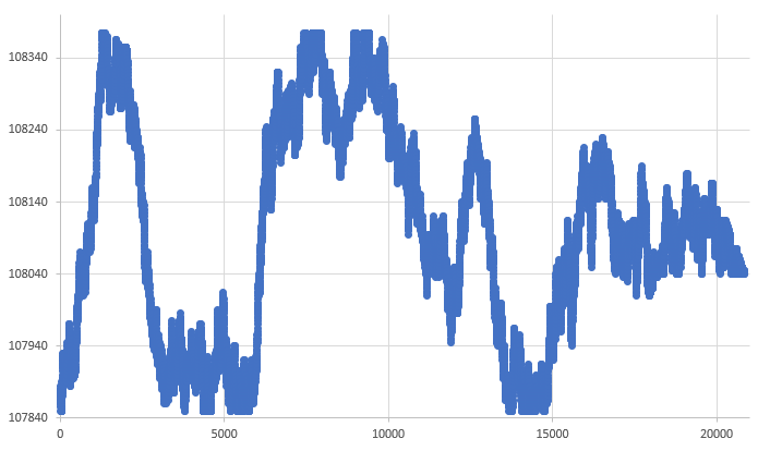
Figure 09 - Random walk with "explosion"
This graph looks much more natural than the graph in Fig. 08. However, even this last graph, which seems perfect, still has a point that is not so natural. It is in the last segment. Pay attention to the end of the graph: it looks somewhat forced, given the limits of possible movement. These things deserve to be fixed, and that's what we'll do now.
To solve this problem, we need to add a few lines to the function responsible for the random walk. Below is the final version of the system:
inline long RandomWalk(long pIn, long pOut, const MqlRates &rate, MqlTick &tick[], int iMode)
                        {
                                double vStep, vNext, price, vHigh, vLow;
                                char i0 = 0;

                                vNext = vStep = (pOut - pIn) / ((rate.high - rate.low) / m_PointsPerTick);
                                vHigh = rate.high;
                                vLow = rate.low;
                                for (long c0 = pIn, c1 = 0, c2 = 0; c0 < pOut; c0++, c1++)
                                {
                                        price = tick[c0 - 1].last + (m_PointsPerTick * ((rand() & 1) == 1 ? -1 : 1));
                                        price = tick[c0].last = (price > vHigh ? price - m_PointsPerTick : (price < vLow ? price + m_PointsPerTick : price));
                                        switch (iMode)
                                        {
                                                case 0:
                                                        if (price == rate.close)
                                                                return c0;
                                                        break;
                                                case 1:
                                                        i0 |= (price == rate.high ? 0x01 : 0);
                                                        i0 |= (price == rate.low ? 0x02 : 0);
                                                        vHigh = (i0 == 3 ? rate.high : vHigh);
                                                        vLow = (i0 ==3 ? rate.low : vLow);
                                                        break;
                                                case 2:
                                                        break;
                                        }
                                        if ((int)floor(vNext) < c1)
                                        {
                                                if ((++c2) <= 3) continue;
                                                vNext += vStep;
                                                if (iMode == 2)
                                                {
                                                        if ((c2 & 1) == 1)
                                                        {
                                                                if (rate.close > vLow) vLow += m_PointsPerTick; else vHigh -= m_PointsPerTick;
                                                        }else
                                                        {
                                                                if (rate.close < vHigh) vHigh -= m_PointsPerTick; else vLow += m_PointsPerTick;
                                                        }
                                                } else
                                                {
                                                        if (rate.close > vLow) vLow = (i0 == 3 ? vLow : vLow + m_PointsPerTick); else vHigh = (i0 == 3 ? vHigh : vHigh - m_PointsPerTick);
                                                }
                                        }
                                }

                                return pOut;
                        }
It seems a little strange, but look at the following: when we execute the first and second segment, the code that will actually be executed looks like this. When we move to the third segment, we will have a slightly different figure.
To get a figure, which in graphical analysis is called SYMMETRICAL TRIANGLE, it is necessary to gradually reduce both sides. But it is very important to understand that we may have a SYMMETRICAL TRIANGLE or ASYMMETRICAL one. Depending on whether the starting point is equidistant between the extreme points, we will have the construction of a symmetrical triangle. If the closing or exit point is very close to one of the boundaries, then the triangle will be asymmetrical. To do this, we will use alternating addition and subtraction. This is done, in particular, at such points. The method of switching data points is implemented by checking the current reduction value.
Thus, we will get a final graph very similar to the graph shown in Fig. 10. It is shown below:
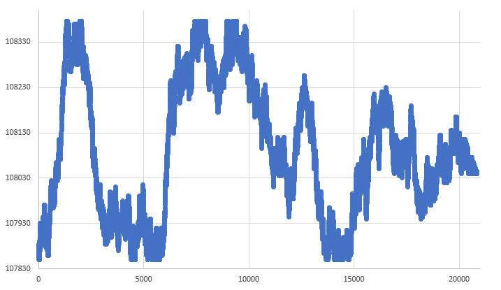
Figure 10 - Random walk graph of a 1-minute bar
It looks much more natural than any other chart we've seen before. Thus, we close the random walk base, and we can move on to the next stages of creating our replay/simulation system.
So you can understand how the system is currently doing.
The attachment contains the complete code in its current state of development.
Conclusion
You don't really need to use complex mathematics to explain or create things. When the wheel was invented, no math was used to determine what its radius should be based on the value corresponding to PI. All we did was achieve the desired movement. In this article, I showed that simple mathematics used in children's games can explain and represent movements that many consider impossible. And they keep using fancy math even though the solution is simple. Always try to make things simple.
Translated from Portuguese by MetaQuotes Ltd.
Original article: https://www.mql5.com/pt/articles/11071
Warning: All rights to these materials are reserved by MetaQuotes Ltd. Copying or reprinting of these materials in whole or in part is prohibited.
This article was written by a user of the site and reflects their personal views. MetaQuotes Ltd is not responsible for the accuracy of the information presented, nor for any consequences resulting from the use of the solutions, strategies or recommendations described.
 The case for using a Composite Data Set this Q4 in weighing SPDR XLY's next performance
- Free trading apps
- Over 8,000 signals for copying
- Economic news for exploring financial markets
You agree to website policy and terms of use