How to catch look-ahead bias in your training set before you train the model
14 October 2026, 21:11

0
36
How to catch look-ahead bias in your training set before you train the model
Building an ONNX-ready dataset inside MetaTrader 5: features, labels and a causality check
Most machine learning failures in trading do not come from a bad model. They come from poisoned
data: information from the future slips into the training set unnoticed. The model looks great on
history and falls apart in live trading.
This note shows how to build a dataset inside MetaTrader 5 and how the built-in check catches the
most common mistake on the way there: normalizing on the whole history. I use the
ARV ML Dataset Export utility and real numbers from an actual run.
The most expensive mistake: normalizing on the whole history
The standard recipe looks like this: collect features, compute the mean and standard deviation over
the whole history, normalize, split into train and test, train the model. The problem is the third
step.
If the mean and standard deviation are computed over the whole history, the features of 2015 bars
already carry information about 2026. Formally the model trains on the past, but in practice it sees
the statistics of the future. Such a solution looks excellent in validation and almost always falls
apart in live trading.
The correct approach is to fit the statistics on the training window only. The natural question then
is how different the training statistics are from the full sample. If the difference is small, the
mistake is harmless. If it is large, full-sample normalization shifts the model noticeably. That
difference is exactly what the utility measures and prints to the journal.
What the utility does
ARV ML Dataset Export is a script for MetaTrader 5. One run on a chart produces two files.
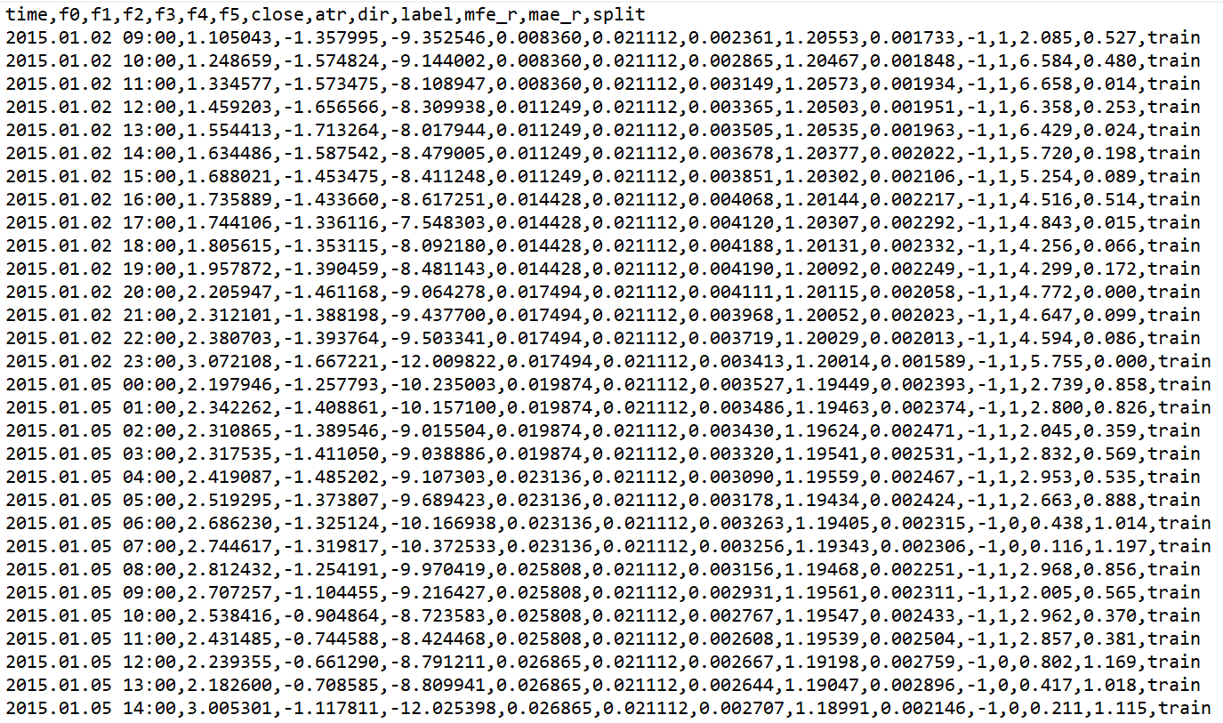
The first is `ARV_ML_<SYMBOL>_H1.csv`: the feature matrix, labels and the train/test split.
| time,f0,f1,f2,f3,f4,f5,close,atr,dir,label,mfe_r,mae_r,split |
Features are computed from the H1, H4 and M15 series of the selected symbol and expressed in ATR
units, so they are comparable across instruments:
f0 = |EMA20(H1) - EMA50(H1)| / ATR14(H1) // distance between averages in volatility units
f1 = (EMA20(H1) - EMA20(H1) 5 bars ago) / ATR14(H1) // momentum: speed of change of EMA20
f2 = (Close(H1) - EMA200(H1)) / ATR14(H1) // deviation of price from the long-term trend
f3 = (BB_upper(H4) - BB_lower(H4)) / EMA20(H4) // Bollinger band width relative to the middle
f4 = ATR14(M15) / Close(M15) * 100 // M15 volatility as a percentage of price
f5 = StdDev20(H1, SMA) / EMA20(H1) // price variability relative to the average
The `label` column is the outcome of a take profit / stop loss race inside a 48-bar H1 horizon: `1`
if TP was reached before SL, `0` if SL came first, empty if neither happened inside the horizon. TP
and SL distances are set in ATR multiples, so labelling does not depend on the volatility of a
particular instrument. The file also carries `mfe_r` and `mae_r`, the maximum favourable and adverse
excursion inside the horizon in R units.
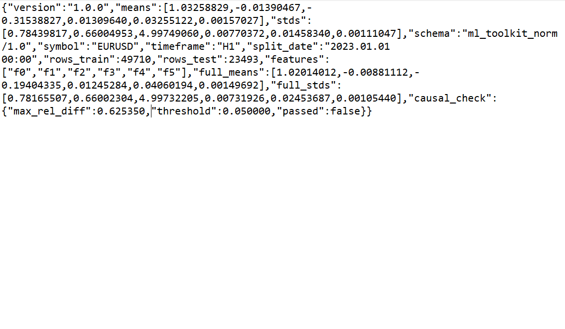
The second file is `ARV_ML_Norm_<SYMBOL>_H1.json`:
version, means[6], stds[6], schema, symbol, timeframe, split_date,
rows_train, rows_test, features[], full_means[6], full_stds[6],
causal_check{max_rel_diff, threshold, passed}
This is where the important part lives: `means` and `stds` are fitted on train rows only, while
`full_means` and `full_stds` are computed on the whole sample. The `causal_check` block compares
them and reports a measurable number, `max_rel_diff`.
How it looks on a real run
EURUSD H1, history from 2015.01.01, train/test boundary at 2023.01.01:
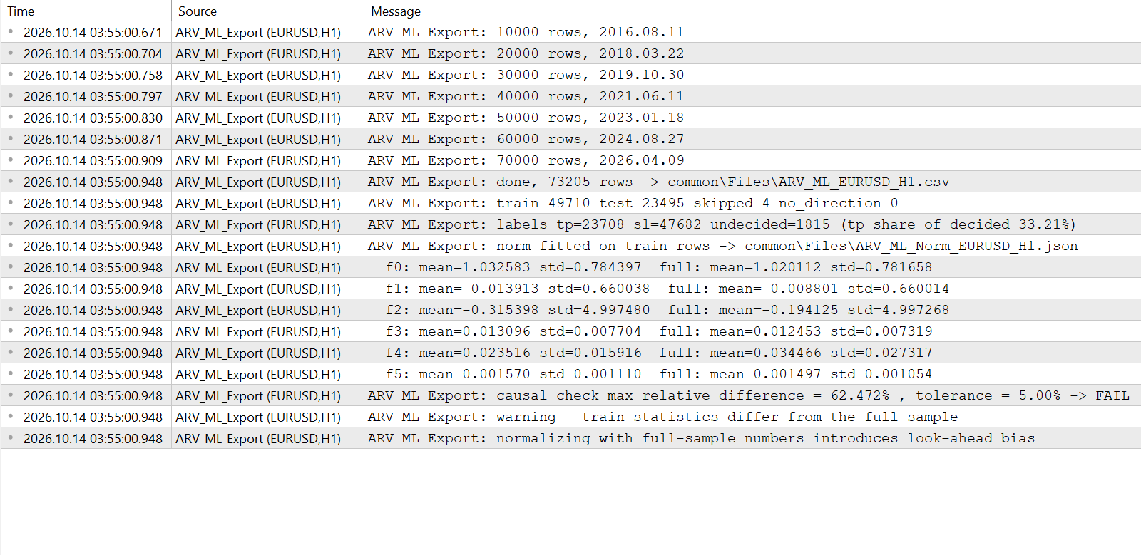
ARV ML Export: done, 73205 rows -> common\Files\ARV_ML_EURUSD_H1.csv
ARV ML Export: train=49710 test=23495 skipped=4 no_direction=0
ARV ML Export: labels tp=23708 sl=47682 undecided=1815 (tp share of decided 33.21%)
ARV ML Export: norm fitted on train rows -> common\Files\ARV_ML_Norm_EURUSD_H1.json
ARV ML Export: causal check max relative difference = 62.472% , tolerance = 5.00% -> FAIL
ARV ML Export: warning - train statistics differ from the full sample
ARV ML Export: normalizing with full-sample numbers introduces look-ahead bias
The key number here is 62.472 %. That is the gap between the training statistics and the full
sample, and it is almost 12.5 times the 5 % threshold. The JSON shows where it comes from:
| Feature | Quantity | On train | On full sample | Relative difference |
|---|---|---|---|---|
| f2 | mean | -0.315398 | -0.194125 | 62.5 % |
| f1 | mean | -0.013913 | -0.008801 | 58.1 % |
| f4 | standard deviation | 0.015916 | 0.027317 | 41.7 % |
Feature `f2` is the deviation of price from EMA200 in ATR units. On the training window its mean is
clearly negative; on the full history it is almost twice as close to zero. The training window lives
in a different market regime, so full-sample normalization would shift its features by roughly two
thirds of their full spread.
One thing not to confuse: `FAIL` in the report is not a bug. It is the useful output. It says that
the full sample and the training window live in different statistical regimes and that full-sample
normalization cannot be used. Had the gap stayed inside the tolerance, the report would have printed
`PASS`.
Split by date, not randomly
Financial series are not independent: neighbouring bars belong to the same market regime, be it a
trend, a range or a news spike. Shuffle the data randomly and the same regimes land in both train
and test at once. The quality estimate becomes inflated and the model overfitted.
That is why the split is done by date: the boundary is set by `InpSplitDate`, and the CSV simply
carries a `split` column with the value `train` or `test`. No extra processing is needed at training
time.
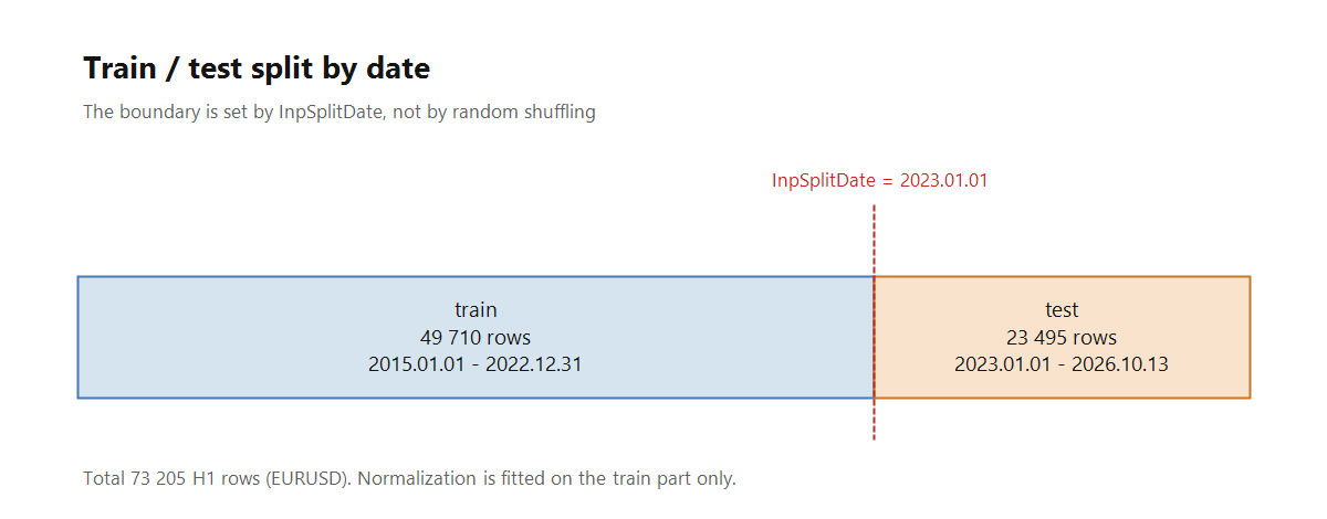
Fig. 1. The train/test boundary is set by `InpSplitDate`; normalization is fitted on the train part only.
What to do with the dataset next
Training is deliberately left outside the terminal. The order is: load the CSV, normalize the
features with `means` and `stds` from the JSON, train any model that can be exported to ONNX, and
load it in MetaTrader 5 with `OnnxCreateFromBuffer`. The format reads equally well in Python with
NumPy and in anything else.
One more thing worth stressing: the dataset itself is not a strategy. Numbers such as the tp/sl
label share describe only what sits in the file and say nothing about future profitability. Any
model trained on this data needs independent out-of-sample validation, and past results do not
guarantee future ones.
What to do next
If you are building an ML approach in trading, check how much the training-window statistics differ
from the full sample. Even if the model is trained outside the terminal, data preparation and the
causality check should be transparent and reproducible. Start simple: compute the mean and the
standard deviation twice, on train only and on the whole history, and compare. If the gap is more
than a few percent, full-sample normalization will already spoil the model.
The ARV ML Dataset Export script is published in the Market.
It runs on MetaTrader 5 build 3000 or later. Pure MQL5: no DLL, no WebRequest, no external services,
and read-only with respect to the account, with no trading operations at all.
Files:
ARV_ML_Export_docs.zip
11 kb
02_journal_report.png
115 kb
03_csv_export.png
125 kb
04_json_causal_check.png
33 kb
ARV_ML_EURUSD_H1_sample.csv
109 kb