The introduction of the Transformer architecture back in 2017 led to the emergence of Large Language Models (LLMs), which demonstrate high results in solving natural language processing problems. Quite soon the advantages of Self-Attention approaches have been adopted by researchers in virtually every area of machine learning.
However, due to its autoregressive nature, the Transformer Decoder is limited by the memory bandwidth used to load and store the Key and Value entities at each time step (known as KV caching). Since this cache scales linearly with model size, batch size, and context length, it can even exceed the memory usage of the model weights.
Transformer architecture-based models demonstrate high efficiency, but their use is complicated by high resource costs both at the training stage and during operation. In this article, I propose to get acquainted with algorithms that allow to reduce memory usage of such models.
In the previous article "Neural network in practice: Straight Line Function", we were talking about how algebraic equations can be used to determine part of the information we are looking for. This is necessary in order to formulate an equation, which in our particular case is the equation of a straight line, since our small set of data can actually be expressed as a straight line. All the material related to explaining how neural networks work is not easy to present without understanding the level of knowledge of mathematics of each reader.
Today we will begin to consider how to implement the calculation of pseudo-inverse in pure MQL5 language. The code we are going to look at will be much more complex for beginners than I expected, and I'm still figuring out how to explain it in a simple way. So for now, consider this an opportunity to learn some unusual code. Calmly and attentively. Although it is not aimed at efficient or quick application, its goal is to be as didactic as possible.
In recent years, many researchers have focused their efforts on studying time series using deep learning models. These methods have proven effective in capturing nonlinear relationships and handling long-term dependencies, which is especially useful for modeling complex systems. However, despite significant achievements, there are still questions of how to efficiently extract and integrate long-term dependencies and short-term features. Understanding and properly combining these two types of dependencies is critical to building accurate and reliable predictive models.
Efficient extraction and integration of long-term dependencies and short-term features remain an important task in time series analysis. Their proper understanding and integration are necessary to create accurate and reliable predictive models.
In the previous article we built the main modules of the MSFformer model, including CSCM and Skip-PAM. The CSCM module constructs a feature tree of the analyzed time series, while Skip-PAM extracts information from time series at multiple scales using attention mechanism based on a temporal feature tree. In this article, we will continue that work by training the model and evaluating its performance on real-world data using the MetaTrader 5 Strategy Tester.
When exploring various model architecture designs, we often devote insufficient attention to the process of model training. In this article, I aim to address this gap.
Piecewise linear representation of time series is a method of approximating a time series using linear functions over small intervals. In this article, we will discuss the algorithm of Bidirectional Piecewise Linear Representation of time series (BPLR), which was presented in the paper "Bidirectional piecewise linear representation of time series with application to collective anomaly detection". This method was proposed to solve problems related to finding anomalies in time series.
This article is somewhat different from my earlier publications. In this article, we will talk about an alternative representation of time series. Piecewise linear representation of time series is a method of approximating a time series using linear functions over small intervals.
The price of a financial instrument represents a highly volatile time series influenced by numerous factors, including interest rates, inflation, monetary policy, and investor sentiment. Modeling the relationship between the price of a financial instrument and these factors, as well as forecasting their dynamics, is a significant challenge for researchers and investors.
We continue the discussion about the use of piecewise linear representation of time series, which was started in the previous article. Today we will see how to combine this method with other approaches to time series analysis to improve the price trend prediction quality.
In the previous article "Neural Network in Practice: Pseudoinverse (I)", I showed how you can use a function available in the MQL5 library to calculate the pseudoinverse. However, the method present in the MQL5 library, as in many other programming languages, is intended to calculate the pseudoinverse when using matrices or at least some structure that may resemble a matrix.
We continue the discussion about the use of piecewise linear representation of time series, which was started in the previous article. Today we will see how to combine this method with other approaches to time series analysis to improve the price trend prediction quality.
Throughout this series of articles, we have explored a variety of architectural approaches for time series modeling. Many of these approaches achieve commendable results. However, it is evident that they do not fully use the advantage of complex patterns present in time series, such as seasonality and trend. These components are fundamental distinguishing characteristics of time series data. Consequently, recent studies suggest that deep learning-based architectures may not be as robust as previously believed, with even shallow neural networks or linear models outperforming them on certain benchmarks.
We continue to study time series forecasting models. In this article, we get acquainted with a complex algorithm built on the use of a pre-trained language model.
In the previous article we got acquainted with the theoretical aspects of the TEMPO method, which proposes an original approach to using pre-trained language models to solve time series forecasting problems. Here's a brief recall of the main innovations of the proposed algorithm.
We continue our acquaintance with the TEMPO method. In this article we will evaluate the actual effectiveness of the proposed approaches on real historical data.
In the previous article Neural Network in Practice: Pseudoinverse (II), I discussed the importance of dedicated computational systems and the reasons behind their development. In this new article related to neural networks, we will delve deeper into the subject. Creating material for this stage is no simple task. Despite appearing straightforward, explaining something that often causes significant confusion can be quite challenging.
What will we cover at this stage? In this series, I aim to demonstrate how a neural network learns. So far, we have explored how a neural network establishes correlations between different data points.
In this article we will build a basic neuron. And although it looks simple, and many may consider this code completely trivial and meaningless, I want you to have fun studying this simple sketch of a neuron. Don't be afraid to modify the code, understanding it fully is the goal.
Allow the use of cookies to log in to the MQL5.com website.
Please enable the necessary setting in your browser, otherwise you will not be able to log in.
You are signed in. Two-factor authentication has been disabled. Set it up again and scan a new QR code, or continue with two-factor authentication disabled.
Neural Networks Made Easy (Part 95): Reducing Memory Consumption in Transformer Models
The introduction of the Transformer architecture back in 2017 led to the emergence of Large Language Models (LLMs), which demonstrate high results in solving natural language processing problems. Quite soon the advantages of Self-Attention approaches have been adopted by researchers in virtually every area of machine learning.
However, due to its autoregressive nature, the Transformer Decoder is limited by the memory bandwidth used to load and store the Key and Value entities at each time step (known as KV caching). Since this cache scales linearly with model size, batch size, and context length, it can even exceed the memory usage of the model weights.
Neural Network in Practice: Pseudoinverse (I)
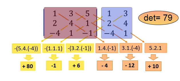
In the previous article "Neural network in practice: Straight Line Function", we were talking about how algebraic equations can be used to determine part of the information we are looking for. This is necessary in order to formulate an equation, which in our particular case is the equation of a straight line, since our small set of data can actually be expressed as a straight line. All the material related to explaining how neural networks work is not easy to present without understanding the level of knowledge of mathematics of each reader.Neural Networks Made Easy (Part 96): Multi-Scale Feature Extraction (MSFformer)
Neural Networks Made Easy (Part 97): Training Models With MSFformer
Neural Networks in Trading: Piecewise Linear Representation of Time Series
Neural Networks in Trading: Dual-Attention-Based Trend Prediction Model
Neural Network in Practice: Pseudoinverse (II)
Neural Networks in Trading: Using Language Models for Time Series Forecasting
Neural Networks in Trading: Practical Results of the TEMPO Method
Neural Network in Practice: Sketching a Neuron
In the previous article Neural Network in Practice: Pseudoinverse (II), I discussed the importance of dedicated computational systems and the reasons behind their development. In this new article related to neural networks, we will delve deeper into the subject. Creating material for this stage is no simple task. Despite appearing straightforward, explaining something that often causes significant confusion can be quite challenging.
What will we cover at this stage? In this series, I aim to demonstrate how a neural network learns. So far, we have explored how a neural network establishes correlations between different data points.