Avoiding Over-fitting in Trading Strategy (Part 2): A Guide to Building Optimization Processes

In the ever-evolving world of automatic trading robot, it is crucial to understand the significance of building an optimization process to avoid the pitfall of over-fitting.

Over-fitting refers to the phenomenon when a trading strategy is excessively tailored to fit historical data, resulting in poor performance when applied to unseen market conditions. It is a common pitfall that can erode the effectiveness and reliability of a trading strategy, leading to potential financial losses.

To counter this issue, it is imperative to establish a robust optimization process. This process involves carefully selecting and testing various parameters, indicators, and models to ensure that the trading strategy remains adaptable and effective across different market conditions.

This article delves into how to building an optimization process to mitigate the risks associated with over-fitting in trading strategies. It also introduces the Anti-Overfitting process that I devised to optimize my trading system.

It is recommended to read Part 1 first in order to comprehend the indications and reasons behind over-fitting.:

- Link 1: Avoiding Over-fitting in Trading Strategy (Part 1): Identifying the Signs and Causes

- Link 2: Tracking the live performance of the strategy used for research here

 

To ensure a robust optimization process, two stages are involved: the Initial Optimization phase for identifying optimal parameter values, and the Walk-forward phase for validating the chosen parameters using new data. Each phase requires different implementation methods and has specific requirements. It is important to note that no historical data used in the Initial Optimization phase is reused in the Walk-forward phase.

 

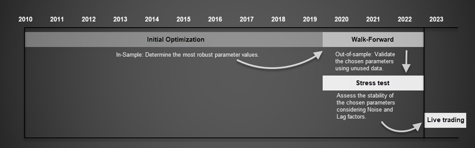
Figure 1. Optimization Process timeline.

The diagram above illustrates the timeline arrangement of these two stages:

- The Initial Optimization phase begins with the earliest available data.

- The Walk-forward phase concludes at the current date.

- The Walk-forward phase begins immediately after the Initial Optimization phase ends.

To determine the allocation of historical data for the Initial Optimization phase, two factors need consideration: (1) the length of available historical data, and (2) the number of parameters to optimize.

To determine the allocation of historical data for the Initial Optimization phase, two factors need consideration: (1) the length of available historical data, and (2) the number of parameters to optimize. The ratio between the two phases depends on the number of parameters being simultaneously optimized. As discussed in Part 1, a higher degrees of freedom necessitates a larger sample size during backtesting to achieve statistical significance. Therefore, if a strategy has more parameters to optimize during the backtest, a larger amount of data is required for the Initial Optimization phase. In the Forward test phase, which is designed to validate the parameters selected from stage 1, the input parameters remain unchanged, resulting in zero degrees of freedom.

Typically, the data ratio between the Initial Optimization phase and Walk-forward phase is 2:1 when optimizing a single parameter, 3:1 when optimizing two parameters, and 4:1 when optimizing three parameters. If the number of parameters exceeds this, it is advisable to divide the strategy into sub-strategies for optimization to avoid the situation that the trading strategy is excessively tailored to historical data, as discussed in Part 1.

Once the Walk-forward phase is completed, Stress Testing is conducted. This stage employs a simulation algorithm to introduce Noise and Lag variables to the entry and exit points determined by the selected parameters from the previous two stages. The purpose is to push the chosen parameters beyond their ''comfort zone'' and assess system's tolerance to random factors such as lag and noise. This serves as the ultimate test to determine if a strategy is suitable for actual trading.

This section provides a detailed explanation of the steps involved in each stage of the optimization process. To facilitate understanding, I will provide practical examples of how I apply this process to extract and validate parameter values for my trading system – Boring Pips.

Trading System Name: Boring Pips

Description of Trading Strategy: The strategy relies on declining price momentum signals at potential support and resistance zones to make trading decisions.

Optimization setting:

- Duration: 12 years and 09 months (01.01.2010 – 31.09.2022)

- Number of parameters optimized (variables) = 2:

• Momentum (open signal)  (13) = 10,15,20,25,30,…65,70.
• Fibonaci level (close signal) (8) = 15,20,25,30,35,40,45,50.

Total parameter combinations: 104.

- Performance Metric: The effectiveness of the strategy in the optimization process is evaluated using the CAGR/MDD (Compound Annual Growth Rate over Max Drawdown).

- Allocate past data for optimization stages: Since there are 2 parameters in the backtest process, the ratio between the Initial Optimization Phase and the Walk-forward Phase is 3:1. Here are the specified time periods for each phase:

• Initial Optimization Phase: January 1, 2010 - May 31, 2019.
• Walk-forward Phase: June 1, 2019 - September 31, 2022.
• Stress Testing: June 1, 2019 - September 31, 2022.

 

Initial Optimization is the first stage of the optimization process, which is also the stage that requires the most historical data.

The objectives of this phase are as follows:

-  Determine whether the strategy has a trading edge and if that edge is significant enough to exploit.

-  Identify the most robust parameter values.

Implementation Process:

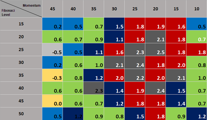
Step 1: Perform a backtest using the 104 sets of input combination parameters with data from 01.01.2010 to 31.05.2019.

Step 2: Calculate the CAGR/MDD for each set of parameters based on the backtest results (Profit and MDD). Aggregate this data into a table.

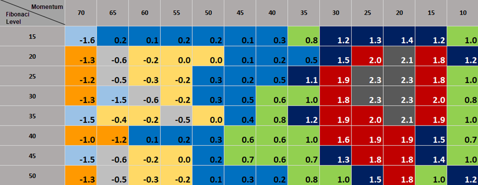
Table 1. CAGR/MDD for each set of parameters based on the backtest results.

 

Note: CAGR is calculated using the formula:

Where:

• Final value is the equity at the end of the backtest.
• Starting value is the equity at the beginning of the backtest.
• N is the duration of the backtest in years.

Step 3: Create a chart from tabular data for a visual and easy-to-analyze overview.

Since the optimization process involves 2 input parameters (Momentum and Fibonacci level) and 1 output parameter (CAGR/MDD), a 3D chart is used as follows. The chart includes:

• x-axis: Momentum (input variable values).
• y-axis: Fibonacci level (input variable values).
• z-axis: CAGR/MDD (output variable value).

 

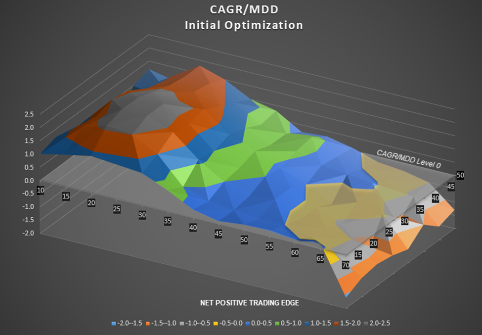
Figure 2. Net Positive Trading Edge chart.

Let's examine this chart and draw a few key observations:

• The profile results seem to have significance, supporting our initial premise that entering reversal orders at potential support/resistance zones during periods of decreasing price momentum leads to improved trading performance. Upon analyzing the chart, we can see that the CAGR/MDD ratio is highest when entering at lower Momentum levels, specifically within the range of 20-25. Additionally, the Fibonacci zone of 25-35 provides the optimal exit signal, although exiting slightly earlier or later still offers trading edge, albeit not as substantial as within this range.
• The majority of the histograms show values above CAGR/MDD = 0, indicating a net positive trading edge.
• The chart exhibits a clear pattern without any erratic nature, providing clear insights into the most successful parameter values.

Based on these observations, we can conclude that when price momentum decrease upon the potential support and resistance areas, entering and exiting orders using appropriate fibonacci levels can offer a trading edge.

Below are 2 examples of chart types of strategies that do not have a trading edge, or a trading edge that is not significant enough to exploit that we can come across when doing optimization.

 

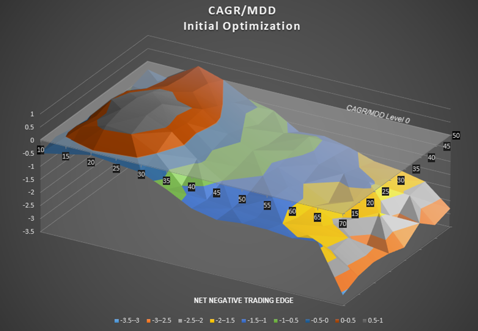
Figure 3. Negative Trading Edge Chart.

This type of chart shows a relationship between momentum and CAGR/MDD, but most of the values fall below level 0, indicating a net negative trading edge. This edge is not significant enough to be exploited effectively.

 

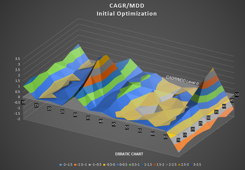
Figure 4. Erract Chart.

Although most of the histograms in this type of chart show values above zero, there is no discernible relationship between the input variable, Momentum, and the output variable, CAGR/MDD. This reveals that the original assumption used to build the trading strategy is incorrect. Trading based on such strategies is risky because there is a fine line between achieving a CAGR/MDD of 3.0 and -2.0.

 

After receiving the backtest results from phase 1, the parameter sets that performed well will undergo a validation process using unseen data.

The objectives of second phase are as follows:

• Evaluating model's power of prediction. To ensure accuracy, none of the data used to build the model in the Initial Optimization phase is reused in this phase.
• Evaluating the compatibility of the trading strategy with current market conditions. The market is constantly changing, and while first phase covers a long historical period to ensure a large sample size, it may not reflect the present market phase. In contrast, Walk-forward phase utilizes a smaller sample size, consisting of data closer to the current period. If a strategy performs well during the Walk-forward phase, it is likely to exhibit similar performance in real trading.

Implementation Process:

Step 1: Out of the 104 parameter sets from stage 1, the top 64 sets will be selected for backtesting in stage 2. These sets include:

• 18 sets for momentum (open signal) with values of 10, 15, 20, 25, 30, 35, 40, and 45.
• 8 sets for Fibonacci levels (close signal) with values of 15, 20, 25, 30, 35, 40, 45, and 50.

Walk-forward period: 01.06.2019 – 31.09.2022.

Performance meter: using the CAGR/MDD to maintain consistency with stage 1.

Step 2: The backtest results will be aggregated into a tabular format.

 

Table 2.  Walk-forward Phase backtest results in tabular format.

 

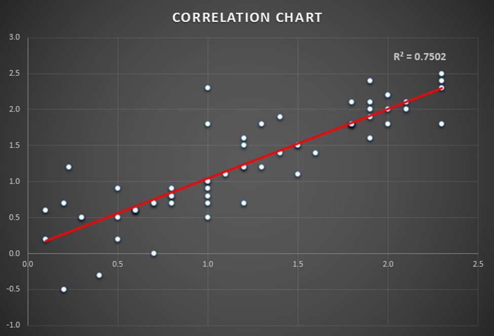
Step 3: A scatter chart will be generated using the collected data to compare the CAGR/MDD values for each parameter set between the Initial Optimization stage and Walk-forward stage. This analysis will help determine the relationship between the strategy's performance between the two phases of in-sample and out-of-sample data..

 

Figure 5. Correlation chart.

The x-axis represents the values from the Initial Optimization and the y-axis represents those values from the Walk-forward phase. Accordingly, when projected onto the x-axis, each white dot represents the CAGR/MDD value of a parameter set during Initial Opitimization, if projected onto the y-axis, it represents the CAGR/MDD value of the parameter set during the Walk-forward test..

From the chart, we can make several observations:

• Initially, most of the parameters show positive CAGR/MDD values during the Walk-forward phase (61/64), indicating that the trading strategy maintains its trading edge in the current market conditions.
• In general, parameter sets that perform well during the Initial Optimization phase also tend to perform well in the Walk-forward test phase, highlighting the predictive ability of the model. There are 2 sets of parameters on the left side of the graph that exhibit negative CAGR/MDD values during the Walk-forward process, these sets of parameters also have low efficiency in the early stages. This can help avoid poor performance parameter sets during live trading.

To quantify this relationship, a trendline can be added with the corresponding R squared value. An R squared value of 0.75 for CAGR/MDD indicates a strong correlation between the performance of a parameter set in the past and its future performance. In other words, the building model has predictive power.

 

Once it has been established that the trading system has an trading edge and the optimal set of parameters has been identified, the Stress testing phase is conducted to assess the tolerance of these parameter values to noise and lag factors.

The original system is modified by introducing noise and lag factors. These factors involve adjusting the entry and exit points of original trades from Walk-forward phase by adding or subtracting a specified price range or time period. The purpose is to evaluate the system's stability under different market conditions, where:

• The Noise variable (N) is used to raise or decrease the price range at the original entry and exit points. This helps assess how the system performs when these points are adjusted by the value of the noise variable.
• The Lag variable (L) is used to add or subtract a time period to the original entry and exit points. This helps evaluate the system's stability when orders are executed later or earlier by the value of the lag variable.

By testing the system's performance under random and unpredictable market conditions, we can determine its sensitivity to changes outside its normal operating range.

It is important to note that this testing process requires basic programming skills to implement. For example, using two-dimentional arrays in the MQL4/MQL5 language to store entry and exit points, as well as adding simulator variables to the system.

Here are the steps to perform stress testing using an Expert Advisor built with the MQL5 language:

Step 1: Use the built-in function OnTester() to save the price and time of all entry/close points during the Walk-forward test.

Step 2: Add the variables Noise (N) and Lag (L) to the original system. Lag represents the time value in minutes that will be added or subtracted from the initial entry and exit points. The L variable also ranges from -30 to +30..

• Noise represents the price range in pips that will be added or subtracted from the initial entry and exit points. The N variable ranges from -30 to +30.
• Lag represents the time value (in minutes) that will be added or subtracted from the initial entry and exit points. The  L variable carries the value from - 30 to + 30.

Step 3: Conduct backtests for each selected parameter set with the trading system that includes the additional noise and delay variables.

Assuming the variable values to be backtested are:

• N (6): -30,-20,-10,10,20,30.
• L (6): -30,-20,-10,10,20,30.

(Note: the combination of N = 0 and L = 0 corresponds to the original backtest result in the Walk-forward process).

And we choose 9 sets of parameters have best CAGR/MDD score from second phase to test, then the sum of the individual backtest results to be performed is 9*60 = 540.

This phase requires processing a large amount of data, so it should only be applied with the highest performance parameter sets found in the previous Walk-forward phase.

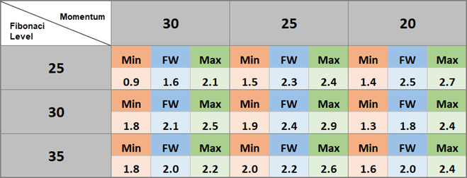
Step 4: Record the results in a table format. For each parameter set, identify the maximum and minimum performance values after applying the noise and lag variables.

 

Table 3. Maximum and minimum performance values after applying the noise and lag variables.

Step 5: Interpret the results using graphs and analysis to gain insights into the system's performance under the Stress testing.

 

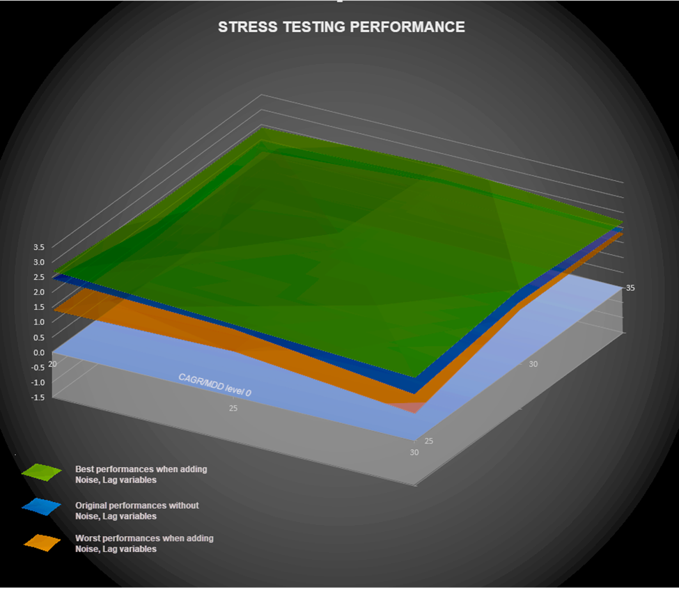
Figure 6. Stress Testing performance.

The results obtained from the Stress testing phase reveal a few key points:

• When setting the highest and lowest performance levels of the parameters under the influence of noise and lag factors on the same chart and comparing them with the initial performance of the Walk-forward phase, the noticeable point is that these three layers of charts all exhibit stable shapes and show no random fluctuations (high/low spikes). This indicates that the parameter sets perform well under noise and lag conditions.
• Additionally, the proximity of the three chart layers suggests the stability of the selected parameter sets. Despite the impact of lag and noise on the entry/exit points of the original positions, the overall performance of the strategy is not significantly affected.
• Even the lowest performance level affected by delay and noise (shown in the orange layer at the bottom) remains above CAGR/MDD = 0, indicating the system's safety. In extreme market conditions, positive performance can still be expected.

 

Final Conclusion

The optimization process described above is designed to eliminate the risk of over-fitting and ensure the generalizability of the trading strategy. Each stage of this process plays a crucial role in optimizing the strategy: Initial Optimization and Walk-forward phase identify the existence of a trading edge based on initial premises and extract the most robust parameter values, while Stress testing phase tests the system's stability against market noise and lag factors.

After undergoing a thorough and comprehensive optimization process, the Boring Pips system has been proven to possess a genuine exploitable trading edge while demonstrating stability in various market conditions, including extreme events. Based on these conclusions, the optimal set of parameters, Momentum (25) and Fibonacci level (30), has been used in actual trading since 10.10.2022. You can find more information about the actual trading performance of the BoringPips strategy at the following link:

Links: Tracking the live performance of the strategy used for research here