Forecasting Financial Time-Series

Introduction

This article deals with one of the most popular practical applications of neural networks, the forecasting of market time-series. In this field, forecasting is most closely related to profitableness and can be considered as one of business activities.

Forecasting financial time-series is a required element of any investing activity. The concept of investing itself - put up money now to gain profits in future - is based on the concept of predicting the future. Therefore, forecasting financial time-series underlies the activities of the whole investing industry - all organized exchanges and other securities trading systems.

Let's give some figures that illustrate the scale of this forecasting industry (Sharp, 1997). The daily turnover of the US stock market exceeds 10 bln US dollars. The Depositary Trust Company in the USA, where securities at the amount of 11 trillion US dollars (of the entire volume of 18 trillion US dollars) are registered, marks approximately 250 bln US dollars daily. Trading world FOREX is even more active. Its daily returns exceed 1000 bln US dollars. It is approximately 1/50 of the global aggregated capital.

99% of all transactions are known to be speculative, i.e., they are not aimed at servicing for real commodity circulation, but are performed to gain profits from the scheme: "bought cheaper and sold better". They all are based on the transactors' predictions about rate changes made. At the same time, and it is very important, the predictions made by the participants of each transaction are polar. So the volume of speculative transactions characterizes the measure of discrepancies in the market participants' predictions, i.e., in the reality, the measure of unpredictability of financial time-series.

This most important property of market time-series underlies the efficient market hypothesis put forth by Louis Bachelier in his thesis in 1900. According to this doctrine, an investor can only hope for the average market profitableness estimated using such indexes as Dow Jones or S&P500 (for New York Exchange). However, every speculative profit occurs at random and is similar to a gamble. The unpredictability of market curves is determined by the same reason for which money can be hardly found lying on the ground in busy streets: there are too many volunteers to pick it up.

The efficient market theory is not supported, quite naturally, by the market participants themselves (because they are exactly in search of this "lying" money). Most of them are sure that market time-series, though they seem to be stochastic, are full of hidden regularities, i.e., they are at least partly predictable. It was Ralph Elliott, the founder of technical analysis, who tried to discover such hidden empirical regularities in the 30's.

In the 80's, this point of view found a surprising support in the dynamical chaos theory that had occurred shortly before. The theory is based on the opposition of chaos state and stochasticity (randomness). Chaotic series only appear random, but, as a determined dynamical process, they leave quite a room for a short-term forecast. The area of feasible forecasts is limited in time by the forecasting horizon, but that may be sufficient to gain real profits due to forecasting (Chorafas, 1994). Then those having better mathematical methods of extracting regularities from noisy chaotic series may hope for a better profit rate - at the expense of their worse equipped fellows.

In this article, we will give specific facts confirming the partial predictability of financial time-series and even numerically evaluate this predictability.

Technical Analysis and Neural Networks

In recent decades, technical analysis - a set of empiric rules based on various market behavior indicators - becomes more and more popular. Technical analysis concentrates on individual behavior of a given security, irrelatively to other securities (Pring, 1991).

This approach is psychologically based on brokers' concentration on exactly the security they are working with at a given moment. According to Alexander Elder, a well-known technical analyst (initially trained as a psychotherapist), the behavior of the market community is very much the same as the crowd behavior characterized by special laws of mass psychology. The crowd effect simplifies thinking, grades down individual peculiarities and produces the forms of collective, gregarious behavior that is more primitive than the individual one. Particularly, the social instinct enhances the role of a leader, an alpha male/female. The price curve, according to Elder, is exactly this leader focusing the market collective consciousness on itself. This psychological interpretation of the market price behavior proves that application of the dynamical chaos theory. The partial predictability of the market is determined by a relatively primitive collective behavior of players that form a single chaotic dynamical system with a relatively small amount of internal degrees of freedom.

According to this doctrine, you have to "break from the bonds" of the crowd, rise above it and become smarter than the crowd to be able to predict the market curves. For this purpose, you are supposed to develop a gambling system evaluated on the previous behavior of a time-series and to follow this system strictly, being unaffected by emotions and rumors circulating around the given market. In other words, predictions must be based on an algorithm, i.e., they can and even must be turned over to a computer (LeBeau, 1992). A man should just create this algorithm, for what purpose he has various software products that facilitate the development and further support of programmed strategies based on technical analysis tools.

According to this logic, why not to use a computer at the strategy development stage, with its being not an assistant calculating the known market indicators and testing the given strategies, but to find optimal indicators and optimal strategies for the indicators found. This approach supported by the application of neural networking technologies has been winning more and more followers since the early 90's (Beltratti, 1995, Baestaens, 1997), since it has a number of incontestable advantages.

First of all, neural network analysis, unlike the technical one, does not assume any limitations on the nature of input data. It can be both the indicators of the given time-series and the information about the behavior of other market securities. Not without reason, these are institutional investors (for example, large pension funds) that actively use neural networks. Such investors work with large portfolios, for which the correlations between different markets are of prime importance.

Second, unlike technical analysis based on general recommendations, neural networks can find indicators optimal for the given security and base on them a forecasting strategy optimal, again, for the given time-series. Moreover, these strategies can be adaptable, changing with the market, which is of prime importance for young, dynamically developing markets, particularly, for the Russian one.

Neural network modeling alone is based only on data without involving any a priori considerations. Therein lies its strength and, at the same time, its Achilles' heel. The available data may be insufficient for learning, the dimensionality of potential inputs may turn out to be too high. Further in this article, we will demonstrate how the experience accumulated by technical analysis can help in overcoming these difficulties, typical in the field of financial predictions.

Time-Series Forecasting Technique

As a first step, let's describe the general scheme of time-series forecasting using neural networks (Fig. 1).

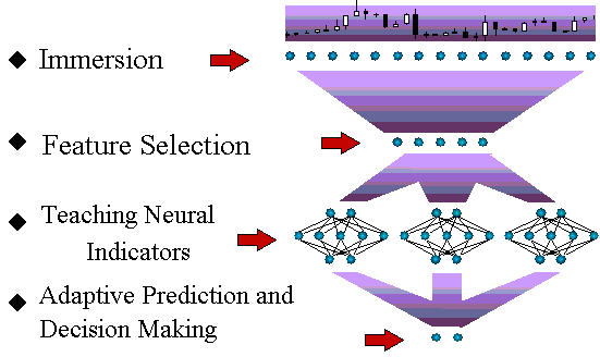
Fig. 1. The Technological Cycle Scheme of Time-Series Forecasting.

Further in this article, we will briefly discuss all stages of this process flow. Although the general principles of neural network modeling are in full applicable to this task, the forecasting of financial time-series has its own specific character. These are these specific features that will be described in this article to the greatest possible extent.

Immersion Technique. Tackens Theorem

Let's start with the immersion stage. As we will now see, for all that predictions seem to be the extrapolation of data, neural networks, indeed, solve the problem of interpolation, which considerably increases the validity of the solution. Forecasting a time-series resolves itself into the routine problem of neural analysis - approximation of a multivariable function for a given set of examples - using the procedure of immersing the time-series into a multidimensional space (Weigend, 1994). For example, a -dimensional lag space of time-series consists of values of the time-series at consecutive instants of time:

.

The following Tackens theorem is proved for dynamical systems: If a time-series is generated by a dynamical system, i.e., the values of are an arbitrary function of the state of such a system, there is such immersion depth (approximately equal to the effective number of degrees of freedom of this dynamical system) that provides an unambiguous prediction of the next value of the time-series (Sauer, 1991). Thus, having chosen a rather large , you can guarantee an unambiguous dependence between the future value of the time-series and its preceding values:, i.e., the prediction of a time-series resolves itself into the problem of multivariable function interpolation. Then you can use the neural network to restore this unknown function on the basis of a set of examples defined by the history of this time-series.

On the contrary, as to a random time-series, the knowledge of the past does not provide any useful hints for predicting the future. So, according to the efficient market theory, the dispersion of the predicted values of the time-series will not change when immersing into the lag space.

The difference between a chaotic dynamics and a stochastic (random) one detected during immersion is shown in Fig. 2.

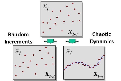
Fig. 2. The difference between a random process and a chaotic dynamics detected while immersing.

Empirical Confirmation of Time-Series Predictability

The immersion method allows us to quantitatively measure the predictability of real securities, i.e., to prove or refute the efficient market hypothesis. According to the latter one, the dispersion of points in all lag space coordinates is identical (if the points are identically distributed independent random values). On the contrary, chaotic dynamics that provides a certain predictability must lead to that observations will be grouped around a certain hypersurface 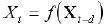, i.e., experimental sample forms a set with the dimension smaller than the dimension of the entire lag space.

To measure the dimensions, you can use the following intuitive property: If a set has the dimension of D, then, provided it is divided into smaller and smaller cubic surfaces with a side of , the number of such cubes will grow as. This fact underlies the detecting the dimension of sets by the box-counting method that we know from previous considerations. The dimension of a set of points is detected by the rate of growing the number of boxes that contain all points of the set. To accelerate the algorithm, we take the dimensions of as multiples of 2, i.e., the resolution scale is measured in bits.

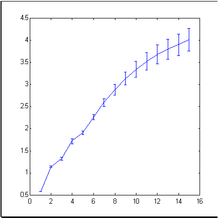
As an example of a typical market time-series, let's take such a well-known financial tool as S&P500 index that reflects the average price dynamics at New York Exchange. Fig. 3 shows the index dynamics for the period of 679 months. The dimension (information dimension is meant) of increments of this time-series, calculated by the box-counting method, is shown in Fig. 4.

Fig. 3. A time-series of 679 values of S&P500, used as an example in this article.		Fig. 4. Information dimension of increments of the S&P500 time-series.

As follows from Fig. 4, the experimental points form a set of the dimension of approximately 4 in a 15-dimensional immersion space. This is much less than 15 that we would obtain based on the efficient market theory which considers the time-series of increments as independent random values.

Thus, the empirical data provide a convincing evidence of the presence of a certain predictable component in financial time-series, although we cannot state that there is a fully determined chaotic dynamics here. Then the attempts to apply neural network analysis for market forecasting are based on strong reasons.

However, it should be noted that theoretical predictability does not guarantee for the attainability of a practically significant level of forecasting. A quantitative estimation of the predictability of specific time-series can be obtained by measuring the cross-entropy, which is also possible using the box-counting technique. For example, we will measure the predictability of S&P500 increments as related to the immersion depth. Cross-entropy

,

the chart of which is given below (Fig. 5), measures the additional information about the next value of the time-series, supported by knowing previous values of this time-series.

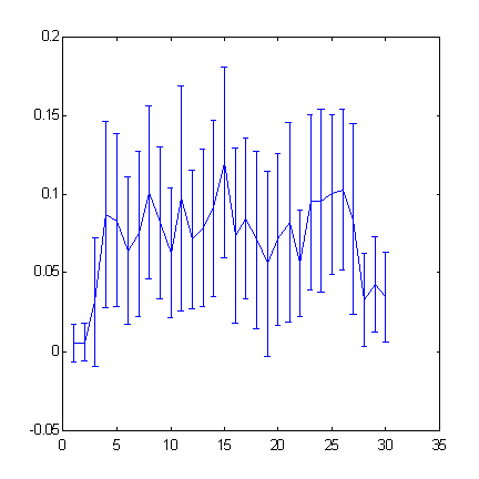
Fig. 5. Predictability of the increment signs for S&P500 time-series as related to the immersion depth (the "window" width).

Increasing immersion depth over 25 will be accompanied by decreasing predictability.

We will further evaluate the profit that is practically reachable at such level of predictability.

Forming an Input Space of Attributes

In Fig. 5, you can see that increasing width of the time-series immersion window eventually results in decreasing predictability - when the increasing input dimensions are not compensated by their information values anymore. In this case, if the lag space dimension is too large for the given number of examples, we have to use special methods of forming a space of attributes with smaller dimensions. The financial-time-series-specific ways of selecting attributes and/or increasing the amount of available examples will be described below.

Choosing Error Functional

To make a neural network learning, it is not sufficient to form teaching sets of inputs/outputs. The network forecasting error must be determined, too. The root-mean-square error used in most neural network applications by default does not have much "financial sense" for market time-series. This is why we will consider in a special section of the article the errors specific for financial time-series and demonstrate how they are related to the possible profit rate.

For example, for choosing a market position, a reliable detection of the sign of the rate changes is much more important than the decrease of the mean square deviation. Though these indications are related to each other, the networks optimized for one of them will provide worse predictions for the other one. Choosing an adequate error function, as we prove it further in this article, must be based on a certain ideal strategy and dictated, for example, by the desire to maximize profits (or minimize possible losses).

Neural Networks Learning

The main specific features of time-series forecasting are in the field of data pre-processing. The teaching procedure for separate neural networks is standard. As usual, the available parameters are divided into three samples: learning, validating and testing. The first one is used for network learning, the second one is for selecting the optimal network architecture and/or for selecting the moment to stop teaching the network. Finally, the third one that has not been used in teaching at all serves for the forecasting quality controlling of the "trained" neural network.

However, for very noisy financial time-series, the use of coterie neural networks may result in significant gaining in prediction reliability. We will end this article with a discussion of this technique.

In some researches, we can find the evidence of better forecasting quality due to the usage of feedback neural networks. Such networks can have a local memory that saves the data of the more distant past than that explicitly available in inputs. However, considering such architectures would make us digressing from the main subject, the more so because there are some alternative methods of efficient expanding the network "horizon" due to special time-series immersion techniques described below.

Forming a Space of Attributes

The efficient coding of inputs is a key to better prediction quality. It is of special importance for hardly predictable financial time-series. All standard recommendations on data pre-processing are applicable here, too. However, there are financial-time-series-specific methods of data pre-processing, we are going to consider in more details in this section.

Time-Series Immersing Methods

First of all, we should keep ion mind that we should not use the values of quotes themselves, which we designate as , as inputs or outputs of a neural network. These are quote changes that are really significant for forecasting. Since these changes lie, as a rule, within a much smaller range than the quotes themselves, there is a strong correlation between the values of rates - the most probable next value of the rate is equal to its preceding value: . At the same time, as it was repeatedly emphasized, to increase the learning quality, we should work for statistical independence of inputs, i.e., for the absence of such correlations.

This is why it is logical to select the most statistically independent values as inputs, for example, quote changes or relative increment logarithm . The latter choice is good for long-lasting time-series, where the inflation affect become quite noticeable. In this case, simple differences in different parts of the series will lie in different ranges, since, in fact, they are measured in different units. On the contrary, the ratios between consecutive quotes do not depend on units of measurement and they will be of the same scale, although the units of measurement change due to inflation. As a result, a greater stationarity of the time-series will allow us to use larger history for teaching and provide a better learning.

A disadvantage of immersing into a lag space is the limited "horizons" of the network. On the contrary, technical analysis does not fix the window in the past and sometimes uses the very far values of the time-series. For example, the maximal and minimal values of a time-series, even taken from a relatively remote past, are asserted to rather strongly affect the traders' psychology and, therefore, these values must still be significant for forecasting. An insufficiently wide window for immersing into the lag space cannot provide such information, which, naturally, decreases the efficiency of forecasting. On the other hand, expanding the window to such values that cover the distant, extreme values of the time-series will increase the network dimensions. This, in its turn, will result in the decreased accuracy of neural network predictions - now due to the network growth.

A way out of this seemingly deadlock situation may be found in alternative methods of coding the past behavior of the time-series. It is intuitively obvious that further the time-series history dates back, the less of its behavior details affect the forecasting results. This is determined by the subjective perception of the past by traders that, strictly speaking, form the future. Therefore, we should find such representation of the time-series dynamics, which would have a selective accuracy: the further to the past, the fewer details. At the same time, the general appearance of the curve must remain intact. The so-called wavelet decomposition can be a very quite promising here. It is equivalent in its information value to the lag immersion, but it makes it easer to compress the data in such a way that the past is described with the selective accuracy.

Decreasing the Dimensions of Inputs: Attributes

This data compression is an example of extracting the attributes most significant for forecasting from an excessively large number of input variables. The methods of systematic extraction of attributes have already been described above. they can (and must) be successively applied to time-series forecasting, too.

It is important that the representation of inputs possibly facilitates the data extraction. The wavelet representation is an example of a good (from the point of view of attributes extraction) coding (Kaiser, 1995). For example, the next graph (Fig. 6) shows a section of 50 values of a time-series with its reconstruction by 10 specially selected wavelet coefficients. Please note that, although it needed five times less data, the immediate past of the time-series is reconstructed accurately, while the remoter past is restored in general outline, highs and lows being reflected correctly. Therefore, it is possible to describe a 50-dimensional window with just 10-dimensional input vector with an acceptable accuracy.

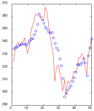
Fig. 6. An example of a 50-dimensional window (solid line) and its reconstruction by 10 wavelet coefficients (o).

Another possible approach is using, as possible candidates for the space of attributes, various technical indicators that are automatically calculated in proper software packages (such as MetaStock or Windows On Wall Street). The great number of such empirical attributes (Colby, 1988) makes their usage difficult, although each of them may turn out to be useful if applied to a given time-series. The methods described above will allow you to select the most significant combination of technical indicators to be used as inputs in the neural network.

Method of Hints

One of the weakest points in financial forecasting is the lack of examples for neural network learning. Generally speaking, financial markets (especially the Russian one) are not stationary. There appear new indexes there for which no history has been accumulated yet, the nature of trading on old markets changes with the time. In these conditions, the length of time-series available for neural network learning is rather limited.

However, we can increase the number of examples by using some a priori considerations about invariants of the time-series dynamics. This is another physico-mathematical term that can considerably improve the quality of financial forecasting. The matter is the generation of artificial examples (hints) obtained from the existing ones through various transformations applied to them.

Let's explain the main idea with an example. The following assumption is psychologically reasonable: traders mostly pay their attention to the shape of the price curve, not to specific values on axes. So, if we stretch the whole time-series a little along the quotes axis, we will be able to use the time-series resulting from such transformation (along with the initial one) for neural network learning. Thus, we have doubled the number of examples due to using a priori information resulting from psychological features of how traders perceive time-series. Moreover, along with increasing the number of examples, we have limited the class of functions to search the solution among, which also increases the prediction quality (if, of course, the invariant used is true to the fact).

The results of calculating the predictability of S&P500 by box-counting method shown below (see Fig. 7, 8) illustrate the role of hints. The space of attributes, in this case, was formed by the orthogonalization technique. We used 30 main components as input variables in the 100-dimensional lag space. Then we selected 7 attributes of these main components - the most significant orthogonal linear combinations. As you can see from Figures below, only application of hints turned out, in this case, to be able to provide a noticeable predictability.

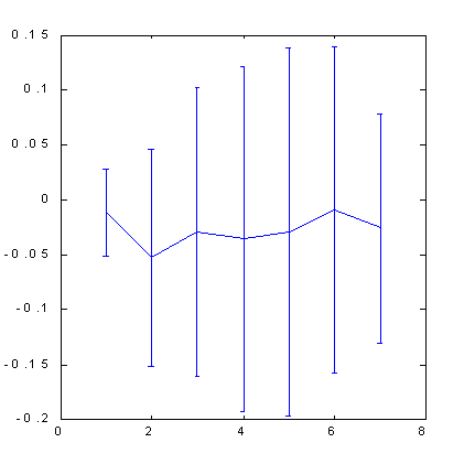Fig. 7. Predictability of quotes change signfor S&P500.

Fig. 8. Predictability of quotes change sign for S&P500 after the number of examples has been quadruplicated by stretching on the price axis.

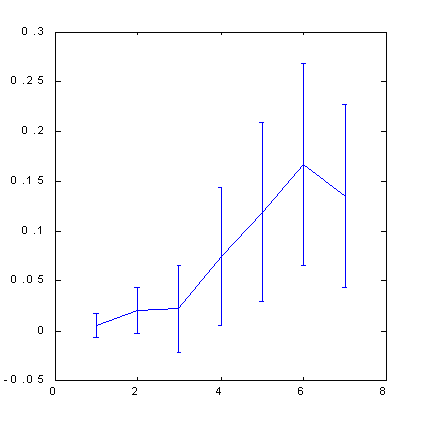
Please note that the use of orthogonal space resulted in a certain increase in predictability as compared to the standard immersion method: from 0.12 bits (Fig. 5) to 0.17 bits (Fig. 8). A bit later, when we start discussing the influence of predictability on profits, we will prove that, due to this, the profit rate can become half as large again.

Another, less trivial example of a successful using such hints for a neural network in what direction to search a solution is the use of hidden symmetry in trading forex. The sense of this symmetry is that forex quotes can be considered from two "viewpoints ", for example, as a series of DM/$ or as a series of $/DM. Increasing of one of them corresponds with decreasing of the other one. This property can be used for doubling the number of examples: add to each example like its symmetric analog . Experiments in neural network forecasting showed that, for basic forex markets, the consideration of symmetry increases the profit rate nearly twice, specifically: from 5% to 10% per annum considering real transaction costs (Abu-Mostafa, 1995).

Measuring the Forecasting Quality

Although forecasting financial time-series resolves itself into the multidimensional function approximation problem, it has its own special features at both forming inputs and selecting outputs for a neural network. We have already considered inputs above. So now let's study the special features of selecting output variables. However, first of all, we should answer the main question: How can the quality of financial forecasting be measured? This will help us find the best neural network learning strategy.

Relation between Predictability and Profit Rate

A special feature of financial time-series forecasting is the working to gaining maximal profits, not to minimizing the mean square deviation, as is the convention in approximation of functions.

In a simplest case of daily trading, profits depend on the correctly predicted sign of the quote changing. This is why the neural network must be aimed at accurate prediction of the sign, not the value itself. Now let's find how the profit rate is related to the sign detecting accuracy in the simplest performance of of daily entering the market (Fig. 9).

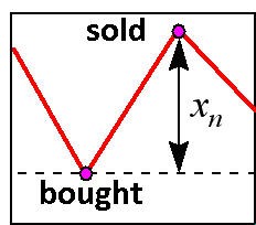
Fig. 9. Daily entering the market.

Let's designate, as of the moment of: the trader's full capital is , relative quote change is , and as the network output let's take its confidence level for the sign of this change: . This network with the output non-linearity of form learns how to predict the change sign and forecasts the sign with the range proportional to its probability. Then the capital gain at step will be recorded as follows:
 

where is the capital share "in play". It is the profit for the entire trading period:

that we will maximize by choosing the optimal rate size . Let the trader correctly predict of signs and, correspondingly, incorrectly predicts with the probability of . Then the profit rate logarithm,

,

and the profit itself will be the highest at the value of and average:

.

Here we have introduced the coefficient of . For example, for Gaussian distribution,. The level of the sign predictability is directly related to cross-entropy that can be estimated a priori by the box-counting method. For binary output (see Fig. 10):

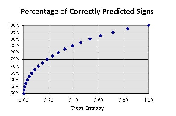
Fig. 10. Fraction of correctly predicted directions of time-series variations as a cross-entropy function of output sign for known inputs.

Eventually, we obtain the following estimation of the profit rate for the given sign predictability value of I expressed in bits:

.
It means that, for the time-series with the predictability of I, it is in principle possible to double the capital within entries to the market. Thus, for example, the previously calculated S&P500 time-series predictability equal to I=0.17 (see Fig. 8) assumes doubling of the capital on average for entries to the market. Thus, even a small quote change sign predictability can provide a very remarkable profit rate.

Here we should emphasize that the optimal profit rate requires a rather careful playing when, at each entry to the market, the player risks a strictly defined share of the capital:

,

where is the profit/loss size typical for this market volatility . Both smaller and larger values of rates will decrease the profit, a too risky trading being able to result in losing money at any predictability. This fact is illustrated in Fig. 11.

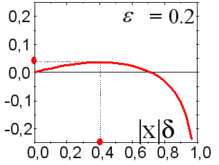
Fig. 11. Dependence of the average profit rate from the selected share of the capital "in the kitty".

This is why the above estimates give an insight into only the upper limit of the profit rate. A more careful study considering the fluctuation effect is beyond the scope of this article. However, it is qualitatively clear that the choice of optimal contract sizes requires the estimation of forecasting accuracy at each step.

Choosing Error Functional

If we take the purpose of forecasting financial time-series to be maximizing the profits, it is logical to adjust the neural network to this final result. For example, if you trade according to the above scheme, you can choose for the neural network learning the following learning error function averaged by all examples from the learning sample:

.

Here, the share of the capital in play is introduced as an additional network output to be adjusted during learning. For this approach, the first neuron, , with activation function will give us the probability of increasing or decreasing rate, while the second network output,, will produce the recommended share of the capital to be invested at the given stage.

However, since this share, according to the preceding analysis, must be proportional to the forecasting confidence level, you can replace two network outputs with only one by placing and limit yourselves to the optimization of only one global parameter,, that will minimize the error:

This produces an opportunity to regulate the rate according to the risk level predicted by the network. Playing with variable rates produces more profits than playing with fixed rates. Indeed, if you fix the rate having defined it by its average predictability, then the capital growth rate will be proportional to , while, if you select the optimal rate at each step, it will be proportional to .

Using Coterie Networks

Generally speaking, the predictions made by different networks trained on the same sample will be different due to the random nature of choosing the initial values of synaptic weights. This disadvantage (an element of uncertainty) can be turned out into an advantage having organized a coterie neural expert consisting of different neural networks. The dispersion of experts' predictions will give an idea of the confidence level of these predictions, which can be used for choosing a correct trading strategy.

It is easy to prove that the average of the coterie values must produce better forecasting than an average expert of the same coterie. Let the error of the ith expert for the input value ofbe equal to. An average error of a coterie is always less than the mean-square error of individual experts in view of Cauchy inequality:

.

It must be noted that the reduction of error can be rather essential. If the errors of individual experts don't correlate with each other, i.e.,, the mean-square error of a coterie consisting of L experts istimes smaller than the average individual error of one expert!

This is why it would be better to base one's forecasting on the average values of the whole coterie. This fact is illustrated by Fig. 12.

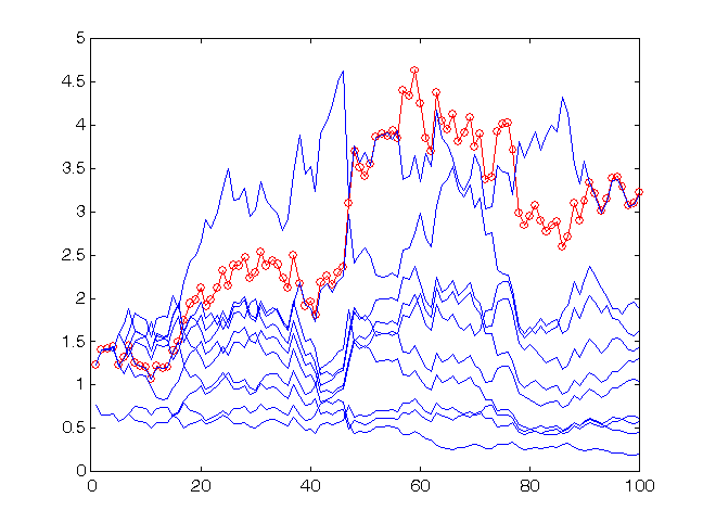
Fig. 12. Profit rate for the last 100 values of time-series sp500 when forecasting with a coterie of 10 networks.

The profit of the coterie (circles) is higher than that of an average expert. The score of correctly predicted signs for the coterie is 59:41.

As you can see from Fig. 12, in this case, the profit of the coterie is even higher than that of each expert. Thus, the coterie method can essentially improve the forecasting quality. Please note the absolute value of profit rate: The capital of the coterie increased 3.25 times at 100 entries to the market (this rate will, of course, be lower if transactional costs are considered).

The predictions were obtained at network learning on the 30 consecutive exponential moving averages (EMA 1 … EMA 30) of the index increment time-series. The increment sign at the next step was predicted.

In this experiment, the rate was fixed at the level of close to the optimal one for the given forecasting accuracy (59 correctly predicted signs vs. 41 incorrectly predicted ones), i.e.,. In Fig. 13, you can see the results of a riskier trading on the same predictions, namely with.

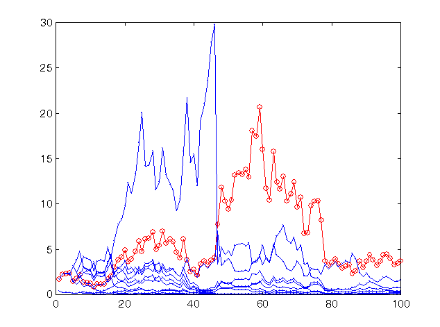
Fig. 13. Profit rate for the last 100 values of time-series sp500 when forecasting with the same coterie of 10 networks, but with a riskier strategy.

The profit of the coterie remains at the same level (a bit increased) since this risk value is as close to optimum as the preceding one. However, for most networks, the predictions of which are less accurate than those of the coterie as a whole, such rates turned out to be too risky, which resulted to their practically full ruining.

The above examples demonstrate how important it is to be able to correctly estimate the forecasting quality and how this estimate can be used to increase the profitability of the same predictions.

We can go to even greater extremes and use the weighted opinions of expert networks instead of the average ones. The weights should be chosen adaptively maximizing the predictive ability of the coterie on the learning sample. As a result, worse trained networks of a coterie make a smaller contribution and don't spoil the prediction.

The possibilities of this method are illustrated by the below comparison of predictions made by two types of coterie networks consisting of 25 experts (see Fig. 14 and 15). The predictions were made according to the same scheme: as inputs, the exponential moving averages of the time-series were used with periods equal to the first 10 Fibonacci numbers. According to the results obtained from 100 experiments, the weighted prediction provides an average excess of correctly predicted signs over the incorrectly predicted ones, approximately equal to 15, while for the average prediction this factor is about 12. It should be noted that the total amount of price rises as compared to declining rates within the given period is exactly equal to 12. Therefore, considering the main tendency to increasing as a trivial constant prediction of the sign of "+" gives the same result for the percentage of correctly predicted signs as the weighted opinion of 25 experts.

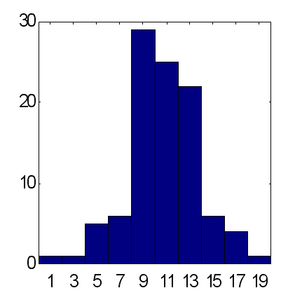
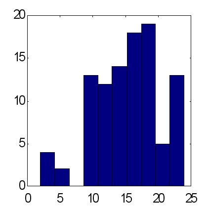
Fig. 14. Histogram of sums of correctly predicted signs at average forecasts of 25 experts. An average for 100 coteries = 11.7 at standard deviation of 3.2.

Fig. 15. Histogram of sums of correctly predicted signs at weighted forecasts of the same 25 experts. An average for 100 coteries = 15.2 at standard deviation of 4.9

Possible Profit Rate of Neural Network Predictions

Up to now, we have formulated the results of numeric experiments as the percentage of correctly predicted signs. Now let's find out about the really reachable profit rate when trading using neural networks. The upper limits of the profit rate, obtained above without considering fluctuations, are hardly reachable in practice, the more so that we have not considered transaction costs before which can cancel out the reached predictability level.

Indeed, considering the commissions results in appearance of a decay constant:

.
Moreover, unlike the predictability level, commission enters linearly, not quadratically. Thus, in the above example, the typical values of predictability cannot exceed commission .

To give an idea of the real possibilities of neural networks in this field, we will give the results of automated trading using neural networks on three indexes with different typical times: the values of index S$P500 with monthly intervals between readings, daily quotes of DM/$, and hourly readings of futures for Lukoil shares on the Russian Exchange. The statistics of forecasting was collected on 50 different neural network systems (containing coteries of 50 neural networks each). The time-series themselves and the results of forecasting the signs on a test set of the last 100 values of each time-series are shown in Fig. 16.

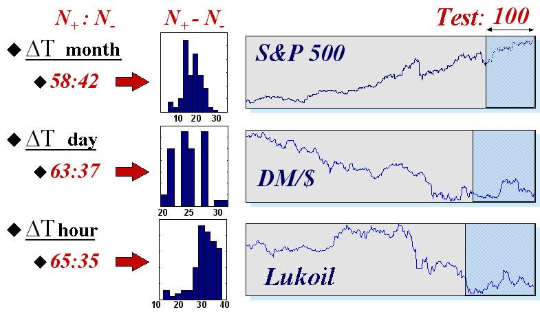
Fig. 16. Average values and histograms of the number of correctly ( ) and incorrectly ( ) predicted signs on testing samples of 100 values of three real financial indexes.

These results confirm the intuitively obvious regularity: the time-series are the more predictable, the less time elapses between the readings. Indeed, the more time passes between the consecutive values of a time-series, the more information, external towards its dynamics, is available for the market participants and, therefore, the less information about the future is in the time-series itself.

Then the predictions obtained above were used for trading on a test set. At the same time, the size of the contract at each step was chosen in proportion to the confidence degree of the prediction, while the value of global parameterwas optimized on the learning sample. Besides, according to its success, each network in the coterie had its own floating rating. In the forecasting at each step, we used only the actually "best" part of networks. The results of such "neural" traders are shown in Fig. 17.

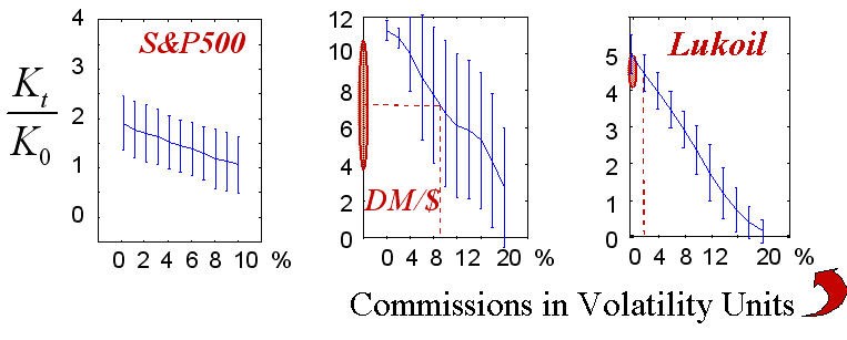
Fig. 17. Winning statistics of 50 realizations according to the amount of commissions.

Real values of commissions drawn in dashed lines show the area of really reachable profit rates.

The final win (like the game strategy itself), of course, depends on the commission size. It is this dependence that is shown in the above diagrams. The realistic values of commissions in the chosen units of measurement known to the author are marked in the figure. It must be refined that the "quantized" nature of the real trading was not considered in those experiments, i.e., we didn't consider that fact that the size of trades must be equal to the integer number of typical contracts. This case corresponds with trading large capitals where the typical trades contain many contracts. Besides, the guaranteed trading was implied, i.e., the profit rate was calculated as a ratio to the security capital that is much smaller than the scaling of contracts themselves.

The above results show that trading based on neural networks is really promising, at least for short terms. Moreover, in view of the self-similarity of financial time-series (Peters, 1994), the profit rate per time unit will be the higher, the less the typical trading time is. Thus, automated traders using neural networks turn out to be most efficient when trading in the real time mode where their advantages over typical brokers are most noticeable: fatigue-proof, nonsusceptibility to emotions, potentially much higher response rate. A well-trained neural network connected to an automated trading system can make decisions much earlier than a human broker recognizes price changes in the charts of his or her terminal.

Conclusion

We demonstrated that (at least some of) market time-series were partly predictable. Like any other kind of neural analysis, the forecasting time-series requires a rather complicated and careful data pre-processing. However, working with time-series has its own specific character that can be used to increase profits. This relates to both the selection of inputs (using special methods of data representation) and the selection of outputs, and the use of specific error functionals. Lastly, we demonstrated how more profitable it is to use coterie neural experts as compared to separate neural networks, and also provided the data of real profit rates on several real securities.

References:

• Sharpe, W.F., Alexander, G.J., Bailey, J.W. (1997). Investments. - 6th edition, Prentice Hall, Inc., 1998.
• Abu-Mostafa, Y.S. (1995). "Financial market applications of learning from hints”. In Neural Networks in Capital Markets. Apostolos-Paul Refenes (Ed.), Wiley, 221-232.
• Beltratti, A., Margarita, S., and Terna, P. (1995). Neural Networks for Economic and Financial Modeling. ITCP.
• Chorafas, D.N. (1994). Chaos Theory in the Financial Markets. Probus Publishing.
• Colby, R.W., Meyers, T.A. (1988). The Encyclopedia of Technical Market Indicators. IRWIN Professional Publishing.
• Ehlers, J.F. (1992). MESA and Trading Market Cycles. Wiley.
• Kaiser, G. (1995). A Friendly Guide to Wavelets. Birk.
• LeBeau, C., and Lucas, D.W. (1992). Technical traders guide to computer analysis of futures market. Business One Irwin.
• Peters, E.E. (1994). Fractal Market Analysis. Wiley.
• Pring, M.G. (1991). Technical Analysis Explained. McGraw Hill.
• Plummer, T. (1989). Forecasting Financial Markets. Kogan Page.
• Sauer, T., Yorke, J.A., and Casdagli, M. (1991). "Embedology". Journal of Statistical Physics. 65, 579-616.
• Vemuri, V.R., and Rogers, R.D., eds. (1993). Artificial Neural Networks. Forecasting Time Series. IEEE Comp.Soc.Press.
• Weigend, A and Gershenfield, eds. (1994). Times series prediction: Forecasting the future and understanding the past. Addison-Wesley.
• Baestaens, D.-E., Van Den Bergh, W.-M., Wood, D. Neural Network Solutions for Trading in Financial Markets. Financial Times Management (July 1994).

The article is published with consent of the author.

About the author: Sergey Shumskiy is the senior research associate at the Physics Institute of the Russian Academy of Sciences, Cand. Sc. (Physics and Mathematics), machine learning and artificial intelligence technician, Presidium member of the Russian Neural Networks Society, the CEO of the IQMen Corp. that develops enterprise expert systems using machine learning technologies. Mr. Shumskiy is a co-author of over 50 scientific publications.

The author's courses: Neural Computing and Its Applications in Economics and Business