Simulink: a Guide for the Developers of Expert Advisors

Introduction

There are several articles which describe the vast possibilities of Matlab. To be more precise, the way that this software is able to expand the programmer's tools, which he uses for developing an Expert Advisor. In this article, I will try to illustrate the work of such a powerful matlab package as the Simulink.

I would like to offer an alternative way to develop automated trading system for traders. I was inspired to turn to this type of method due to the complexity of the problem that the trader faces - the creation, verification, and testing of the automated trading system. I am not a professional programmer. And thus, the principle of "going from the simple to the complex" is of primary importance to me in development of automated trading system. What exactly is simple for me? First of all, this is the visualization of the process of creating the system and the logic of its functioning. Also, it is a minimum of handwritten code. These expectations are quiet consistent with the capabilities of the Simulink® package, a well known MATLAB product, which is a world leader amongst the instruments for visualization of mathematical calculations.

In this article, I will attempt to create and test the automated trading system, based on a Matlab package, and then write an Expert Advisor for MetaTrader 5. Moreover, all of the historical data for backtesting will be used from MetaTrader 5.

To avoid terminological confusion, I will call the trading system, which functions in Simulinik, with a capacious word MTS, and the one which functions in MQL5, simply an Expert Advisor.

1. The fundamentals of Simulink and Stateflow

Before we proceed with specific actions, it is necessary to introduce some form of a theoretical minimum.

With the help of the Simulink® package, which is a part of MATLAB, the user can model, simulate and analyze dynamic systems. In addition, it's possible to raise the question about the nature of the system, to simulate it, and then to observe what occurs.

With Simulink, the user can build a model from scratch or modify an already existing model. The package supports the development of linear and nonlinear systems, which are created on the basis on discrete, continuous and hybrid behavior.

The main properties of the package are presented on the developer's site:

• Extensive and expandable libraries of predefined blocks;
• Interactive graphical editor for assembling and managing intuitive block diagrams;
• Ability to manage complex designs by segmenting models into hierarchies of design components;
• Model Explorer to navigate, create, configure, and search all signals, parameters, properties, and generated code associated with your model;
• Application programming interfaces (APIs) that let you connect with other simulation programs and incorporate hand-written code;
• Embedded MATLAB™ Function blocks for bringing MATLAB algorithms into Simulink and embedded system implementations;
• Simulation modes (Normal, Accelerator, and Rapid Accelerator) for running simulations interpretively or at compiled C-code speeds using fixed- or variable-step solvers;
• Graphical debugger and profiler to examine simulation results and then diagnose performance and unexpected behavior in your design;
• Full access to MATLAB for analyzing and visualizing results, customizing the modeling environment, and defining signal, parameter, and test data;
• Model analysis and diagnostics tools to ensure model consistency and identify modeling errors.

So let us begin the immediate review of the Simulink environment. It is initialized from an already open Matlab window in two of the following ways:

1. by using the Simulink command in the command window;
2. by using the Simulink icon on the toolbar.

Figure 1. Initialization of Simulink

When the command is executed, the libraries browsing window (Simulink Library Browser) appears. 

Figure 2. Library Browser

The browser window contains a tree of Simulink libraries components. To view a particular section of the library, you simply need to select it with the mouse, after which a set of icon components, of the active section of the library, will appear in the right section of the Simulink Library Browser window. Fig. 2 shows the main section of the Simulink library.

Using the browser menu or the buttons of its toolbar, you can open a window to create a new model or to upload an existing one. I should note that all work with Simulink occurs along with an open MATLAB system, in which it's possible to monitor the execution of operations, as long as their output is provided for by the modeling program.

Figure 3. Simpulink blank window

First of all, let us change a few parameters of our model. Let's open Simulation --> Configuration Parameters. This window has a number of tabs with many of parameters. We are interested in the default Solver tab, where you can set the parameters of the solver of the Simulink modeling system.

In the Simulation time the modeling time is set by the beginning time - Start time (usually 0), and the ending time - Stop time.

For our task, let's assign the Start time a value of 1. We will leave the Stop time as is.

In the solver's options, I also changed the Type to Fixed-step, the solver itself to for discrete, and the step (fixed-step size) to 1.

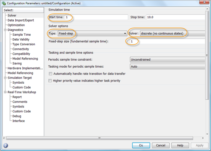
Figure 4. Configuration Parameters Window

The Simulink environment is successfully completes by the subsystem Stateflow, which is an event-driven modeling package, based on the theory of finite-state automates. It allows us to represent the work of the system, based on a chain of rules, which specify the events and actions as response to these events.

The graphical user interface of Stateflow package has the following components:

• A Graphics Editor of SF-charts;
• Stateflow Explorer;
• Stateflow Finder to search for the necessary objects in the SF-charts;
• A debugger of SF-models;
• Real Time Workshop, a real-time code generator.

The most commonly used block diagram (Chart), which is located in the Stateflow section. Let's examine it.

Let's move the block from the library and double click on it to open the diagram. A blank window of an SF-chart editor will appear. It can be used to create SF-charts and their debugging, in order to obtain the needed functions.

The Toolbar is located upright on the left side. There are 9 buttons:

1. State;
2. History Junction;
3. Default Transition;
4. Connective Junction;
5. Truth Table;
6. Function;
7. Embedded MATLAB Function;
8. Box;
9. Simulink Function Call.

Unfortunately, it is impossible to consider every element in detail within the context of this article. Therefore, I will limit myself to a brief description of those elements, which we will be needing for our model. More detailed information can be found in the Matlab Help section, or on the website of the developer.

Figure 5. The view of the SF-chart in the editor

The key object of the SF-charts is the State. It is presented by a rectangle with rounded corners.

It can be exclusive or parallel. Every state may be the parent and has heirs. The states can be active or non-active, the states can perform certain procedures.

The transition is represented as a curved, arrowed line, it connects the states and other objects. A transition can be made by clicking with the left button of your mouse on the source object and by directing the cursor to the target object. The transition may has its own conditions, which are recorded in the brackets. The transition procedure is indicated within the brackets, it will be executed if condition is satisfied. The procedure, executed during the confirmation of the target object, is denoted by a slash.

The alternative node (connective junction) has form of a circle, and allows the transition to way through the different paths, each of which is defined one by a specific condition. In such a case, the transition, which corresponds to the specified condition, is selected.

The function represented as a flow graph with the statements of the Stateflow procedural language. A flow graph reflects the logical structure of use of transitions and alternative nodes.

An Event is another important object of Stateflow, belonging to the group of non-graphic objects. This object can launch the procedures of the SF-chart.

The procedure (action) is also non-graphic object. It can call the function, assign a specific event, transition, etc.

The Data in the SF-model is represented by numeric values. The data is not represented as graphical objects. They can be created at any level of the model's hierarchy and have properties.

2. Description of the Trading Strategy

Now, briefly about the trading. For our training purposes, the Expert Advisor will be very simple, if not to say, primitive.

The automated trading system will open positions on the basis of the signal, basically, after the crossing of the Exponential Movings, with a period of 21 and 55 (Fibonacci numbers), averaged on close prices. So if the EMA 21 crosses up the EMA 55 from the bottom, a long position is opened, otherwise - a short one.

For noise filtering, position will be opened at the K-th bar by the price of the bar opening after the appearance of the 21/55 cross. We will trade on the EURUSD H1. Only one position will be opened. It will be closed only upon reaching the Take Profit or Stop Loss level.

I would like to mention that during the development of automated trading system and the history backtesting, certain simplifications of the overall trade picture are admitted.

For example, the system will not check the broker execution of a signal. Further we will add the trading restrictions to the core of the system in MQL5.

3. The modeling of a Trading Strategy in Simulink

To begin with, we need to upload the historical price data into the Matlab environment. We will do it using a MetaTrader 5 script, which will save them (testClose.mq5).

In Matlab, these data (Open, High, Low, Close, Spread) will be also loaded using a simple m-script (priceTxt.m).

Using the movavg (standard Matlab function) we will create arrays of Exponential Moving Averages:

[ema21, ema55] = movavg(close, 21, 55, 'e');

As well as an auxiliary array of the bar indexes:

num=1:length(close);

Let's create the following variables:

K=3; sl=0.0065; tp=0.0295;

Let's begin the modeling process.

Create a Simulink blank window and call it mts when saving it. All of the following actions have been duplicated in a video format. If something is not quite clear, or even not clear at all, you can look my actions by watching the video.

When saving the model, the system may print the following error:

??? File "C:\\Simulink\\mts.mdl" contains characters which are incompatible with the current character encoding, windows-1251. To avoid this error, do one of the following:
1) Use the slCharacterEncoding function to change the current character encoding to one of: Shift_JIS, windows-1252, ISO-8859-1.
2) Remove the unsupported characters. The first unsupported character is at line 23, byte offset 15.

To eliminate this, you simply need to close all of the models' windows, and change the encoding by using the following commands:

bdclose all
set_param(0, 'CharacterEncoding', 'windows-1252');

Let's specify the information source of our model.

The role of such information source will be the historical data from MetaTrader 5, which contain the opening, maximum, minimum, and closing prices. In addition, we will take into account the Spread, even though it became floating relatively recently. Finally, we record the opening time of the bar. For modeling purposes, some arrays of initial data will be interpreted as a signal, that is as a vector of values of a time function at discrete points in time.

Let's create a "FromWorkspace" subsystem to retrieve the data from the Matlab workspace. Select the Ports & Subsystems section in Simulink libraries browser. Drag the "Subsystem" block to the Simulink model window, using the mouse. Rename it to "FromWorkspace", by clicking on the Subsystem. Then, log into it by double-clicking the left mouse button on the block, in order to create the input and output variables, and the constants for the system.

To create the signal sources in the Library Browser, choose the Signal Processing Blockset, and sources (Signal Processing Sources). Using your mouse, drag the "Signal from Workspace" block into the subsystem window of the FromWorkspace model. Since the model will have 4 input signals, we simply duplicate the block, and create 3 more copies of it. Let's specify right away which variables will be processed by block. To do this, click twice on the block, and input the variable name into the properties. These variables will be: open, ema21, ema55, num. We will name the blocks the following: open signal, ema21 signal, ema55 signal, num signal.

Now, from the "Commonly used blocks" Simulink section, we will add a block for creating a channel (Bus Creator). Open the block and change the number of inputs to 4. Connect the open signal, ema21 signal, ema55 signal, num signal blocks with the inputs of the Bus Creator block.

In addition, we will have 5 more input constants. The "Constant" block is added from the section "Commonly used blocks". As the value (Constant value), we specify the names of the variables: spread, high, low, tp, sl:

• spread - this is an array of spread values;
• high - this is an array of maximum price values;
• low - this i's an array of minimum price values;
• tp - Take Profit value in absolute terms;
• sl - the Stop Loss value in absolute terms.

We will call the blocks as following: spread array, high array, low array, Take Profit, Stop Loss.

Select the output port block (Out1) in the "Ports & Subsystems" Simulink section and move it to the subsystem window. Make 5 copies of the output port. The first one, we'll connected with the Bus Creator block, and others - alternately, with the arrays spread, high, low, Take Profit, and Stop Loss blocks.

We'll rename the first port to price, and the others - by the name of the output variable.

To create a trading signal, let's insert the block of addition (Add) from the Simulink section "Mathematical Operations". We'll call it emas differential. Within the block we will change the list of signs, c + + to + -. Using the Ctrl+ K key combination, turn the block by 90 ° clockwise. Connect the ema21 signal block to the "+" input, and the ema55 signal with the "-". 

Then insert the Delay block, from the Signal Processing Blockset section, of Signal Operations. We'll name it K Delay. In the Delay (samples) field of this block we enter the name of the K variable. Connect it with the previous block.

The emas differential blocks and K Delay format the front (level difference) of the control signal for calculations only for the stage of modeling, where there has been change. The subsystem, which we'll create a little later, will be activated if at least one element has a change in its signal level.

Then, from the Simulink "Commonly used blocks" section, we will add a multiplexer with and (Mux) block. Similarly, rotate the block by 90 ° clockwise. We will split the signal line of the delay block in two, and connect it with the multiplexes.

From the Stateflow section, insert a Chart block. Enter the chart. Add 2 incoming events (Buy and Sell), and 2 outgoing events (OpenBuy and OpenSell). The trigger value (Trigger) for the Buy event, we will set to Falling (activation of the subsystem by a negative front), and for the Sell events, we will set to Rising (activation of the subsystem by a positive front). The trigger value (Trigger) for the events OpenBuy and OpenSell, we will set to the position of Function call (Calling), (activation of the subsystem will be determined by the logic of the work of the given S-function).

We'll create a transition by default with 3 alternative nodes. The first node we will connect by a transition to the second node, setting the conditions and the procedure for them to Buy {OpenBuy;}, and for the third, setting the procedure to Sell {OpenSell;}. Connect the chart input with the multiplex, and the two outputs - with another multiplex, which can be copied from the first. The last block will be connected to the output port, which we will copy from an analogous one, and call it Buy/Sell.

And I almost forgot! For the model to work properly, we need to create a virtual channel object, which will be located in the Matlab workspace. To do it, we enter the Bus Editor via the Tools menu. In the editor, select the item Add Bus. Call it InputBus.

Insert the elements according to the names of the input variables: open, ema21, ema55 and num. Open the Bus Creator and check the checkbox next to Specify properties via bus object (Set the properties through the bus object). In other words, we connected our block with the virtual channel object we created. The virtual channel means that the signals are combined only graphically, without affecting the distribution of memory.

Save the changes in the subsystem window. This concludes our work with the FromWorkspace subsystem.

Now comes the time to create the "Black Box". It will be a block, based on the incoming signals, it will process the information and make trading decisions. Of course, it needs to be created by us, rather than a computer program. After all, only we can decide on the conditions, under which the system should make a trade. In addition, the block will have to display the information about the completed  deals in the form of signals.

The needed block is called the Chart and located in the Stateflow section. We have already been acquainted with it, have we not? Using the "drag and drop" we move it to our model window.

Figure 6. The blocks of the input subsystem and the StateFlow chart

Open the chart and input our data into it. First of all, let's create a channel object, as we have done in the FromWorkspace subsystem. But unlike the former, which supplied us with the signals from the workspace, this one will return the obtained result. And so, we will call the object OutputBus. Its elements will become: barOpen, OpenPrice, TakeProfit, StopLoss, ClosePrice, barClose, Comment, PositionDir, posN, AccountBalance.

Now we will begin constructing. In the chart window, we will display the default transition (# 1).

For the conditions and procedures we shall indicate:

[Input.num>=56 && Input.num>Output.barClose] {Output.barOpen=Input.num;i = Input.num-1;Output.posN++;}

This condition means that the data will be processed if the number of input bars will be at least 56, as well as if the input bar will be higher than the closing bar of the previous position. Then, the opening bar (Output.barOpen) is assigned the number of the incoming bar, by an index variable of i - the index (starting from 0), and the number of the open positions increases by 1.

The 2nd transition is executed only if the open position will not be the first one. Otherwise, the third transition is executed, which will assign the account balance variable (Output.AccountBalance) the value 100000.

The 4th transition is executed if the chart was initiated by the OpenBuy event. In such case, the position will be directing to the purchase (Output.PositionDir = 1), the opening price will become equal to the opening bar price, taking into account the spread (Output.OpenPrice = Input.open + spread [i] * 1e-5). The values of the output signals StopLoss and TakeProfit will also be specified.

If an OpenSell event occurs, then the flow will follow the 5th transition and set its values for the output signals.

The 6th transition is realized if the position is long, otherwise the flow follows to the 7th transition.

The 8th transition checks whether or not the maximum bar price has reached the Take Profit level, or if the minimum bar price has reached the level of Stop Loss. Otherwise, the value of the index variable i is increased by one (9th transition).

The 10th transition verifies the conditions arising at the Stop Loss: the price minimum of the bar has crossed the Stop Loss level. If it's confirmed, the flow will follow to the 11-th transition, and then on to the 12th, where the values of the price differences of the closing and opening positions, the current account balance, and index of the closing bar are defined.

If the 10th transition is not confirmed, then the position will be closed at the Take Profit (13th transition). And then, from the 14th, the flow will follow to the 12-th transition.

The procedures and conditions for the transitions for a short position are the opposite.

Finally, we've created new variables in the chart. In order to automatically integrate them into our model, we need to run the model directly in the chart window, by clicking the "Start Simulation" button. It looks similar to the "Play" button on music players. At this point, the Stateflow Symbol Wizard (SF master objects) will launch, and it will suggest to save the created objects. Press the SelectAll button and then click Create button. Objects have been created. Let us now open the Model Browser. On the left, click on our Chart in the Model Hierarchy. Let's sort out the objects by the data type (DataType).

Add more data by using the "Add" and "Data" menu commands. We'll call the first variable Input. Change the value of the Scopes to Input, and the Type - to "Bus: <bus object name> . And then enter the name, of the earlier created channel, InputBus, right into this field. Thus our Input variable will be have the type of InputBus. Let's set the value of the Port to one.

Complete the same operation with the Output variable. Only it must have the Output Scope and the Output Bus type.

Let's change the scope for the variables high, low, sl, tp, and spread to the value of "Input". Respectively, we will set the port numbers in the following order: 3, 4, 6, 5, 2.

Also let's change the scope of the variable Lots to Constant. On the "Value Attributes" tab let's input 1, OpenBuy and OpenSell events - for Input in the field "Initial" (on the right).  In the events, change the trigger value for the "Function call").

Create an internal variable len, with a Constant scope. On the "Value Attributes" tab, in the "Initial value" field, we'll input an m-function length (close). Thus it will be equal to the length of the close array, which is located in the Matlab workspace.

For the high and low variables we'll input a value of [len 1] into the Size field. Thus, in the memory, we have reserved the array sizes of high and low as the value of [len 1].

Also, let's indicate for the variable K on the "Value Attributes" tab, in the "Initial value" field (on the right) the actual variable of K, taken from the workspace.

As a result, we have a Chart subsystem, with 7 input ports and one output port. Let's position the block in such a way, so that the input events () port was at the bottom. We'll rename the "Position handling" block. In the chart itself, we'll also display the name of the block. Combine the blocks of the FromWorkspace subsystem and the "Position handling" through the appropriate ports. And change the color of the blocks.

It must be noted, that the "Position handling" subsystem will only function if it is "woken up" by incoming OpenBuy or OpenSell events. This way, we optimize the operation of the subsystem to avoid the unnecessary calculations.

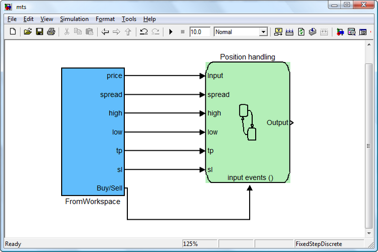
Figure 7. FromWorkspace and Position handling Subsystems

Now we have to create a subsystem to print the processing results in the Matlab workspace and combine it with the "Position handling" subsystem. It will be the easiest task.

Let's create a "ToWorkspace" subsystem for obtaining the results into the workspace. Repeat the steps which we took when we created the "FromWorkspace" subsystem. In the library browser, select the Simulink Ports & Subsystems section. Using the mouse, drag the "Subsystem" block into the Simulink model window. Rename it to "ToWorkspace" by clicking on the "Subsystem". Combine the block with the "Position handling" subsystem.

In order to create the variables log into it by double-clicking on the block with the left mouse button,

Since the subsystem will be receiving data from the OutputBus object, which is a nonvirtual bus, then we need to select the signals from this channel. To do it, we select the Simulink "Commonly used blocks" section in the library Browser, and add a "Bus Selector". The block will have 1 input and 2 output signal, whereas we need to have 10 of such signals.

Let's connect the block to the input port. Press the "Start simulation" button (this is our "Play" button). The compiler will begin to build the model. It will not be built successfully, but it will create input signals for the bus selecting block. If we enter the block, we will see the needed signals appear in the left hand side of the window, which are transmitted via OutputBus. They all need to be selected, using the "Select" button, and move them to the right side - "Selected signals".

Figure 8. Bus Selector block parameters

Let us again refer to the "Commonly used blocks" section of the Simulink libraries browser, and add the Mux multiplex block. It indicates the number of inputs, which is equal to 10.

Then log into the "Sinks" section of the Simulink library Browser, and move the ToWorkspace block to the subsystem window. In there we will indicate the new name of the variable "AccountBalance," and change the output format (Save format) from the "Structure" to the "Array". Combine the block with the multiplex. Delete the output port, since it will no longer be necessary. Customize the color of the blocks. Save the window. The subsystem is ready.

Before constructing the model, we should verify the presence of the variables in the workspace. The following variables must be present: InputBus, K, OutputBus, close, ema21, ema55, high, low, num, open, sl, spread, tp.

Let's set the Stop Time value as the parameter to define num (end). Meaning the processed vector will have the length, which was set by the last element of the num array.

Prior beginning building a model, we need to choose a compiler, using the following command:

mex-setup

Please choose your compiler for building external interface (MEX) files:
Would you like mex to locate installed compilers [y] / n? y

Select a compiler:

[1] Lcc-win32 C 2.4.1 in C:\PROGRA~2\MATLAB\R2010a\sys\lcc
[2] Microsoft Visual C++ 2008 SP1 in C:\Program Files (x86)\Microsoft Visual Studio 9.0
[0] None

Compiler: 2

As you can see, I selected the Microsoft Visual C ++ 2008 compiler SP1.

Let's begin building. Press the "Start simulation" button. There is an error: Stateflow Interface Error: Port width mismatch. Input "spread"(#139) expects a scalar. The signal is the one-dimensional vector with 59739 elements.

The variable "spread" should not have the type double, but rather inherit its type from the signal from Simulink.

In the Model Browser, for this variable, we specify "Inherit: Same as Simulink", and in the Size field, and specify "-1". Save the changes.

Let's run the model again. Now the compiler works. It will show some minor warnings. And in less than 40 seconds the model will process the data of nearly 60,000 bars. Trade is performed from '2001 .01.01 00:00 'to '2010 .08.16 11:00'. The total amount of open positions is 461. You can observe how the model works in the following clip .

4. Implementation of the Strategy in MQL5

And so, our automated trading system is compiled in Simulink. Now we need to transfer this trading idea into the MQL5 environment. We had to deal with Simulink blocks and objects, through which we expressed the logic of our trading Expert Advisor. The current task is to transfer the logic trading system into the MQL5 Expert Advisor.

However, it should be noted that some blocks do not necessarily have to be in some way defined in the MQL5 code, because their functions could be hidden. I will try to comment with a maximum amount of details about which line relates to which block, in the actual code. Sometimes this relationship may be indirect. And sometimes it can reflect an interface connection of blocks or objects.

Before I begin this section, let me to draw your attention to an article "Step by Step Guide to writing Expert Advisors in MQL5 for Beginners". This article provides an easily graspable description of the main ideas and basic rules of writing an Expert Advisor in MQL5. But I will not dwell on them now. I will use some lines of MQL5 code from there.

4.1 "FromWorkspace" Subsystem

For example, we have an "open signal" block in the "FromWorkspace" subsystem. In Simulink, it is needed in order to obtain the opening bar price during backtesting, and to open a position at this price, in case a trading signal is received. This block is obviously not present in the MQL5 code, because the Expert Advisor requests the price information immediately after receiving the trading signal.

In the Expert Advisor we will need to process data, received from moving averages. Therefore, we will create for them dynamic arrays and corresponding auxiliary variables, such as handles.

int ma1Handle;  // Moving Average 1 indicator handle: block "ema21 signal"
int ma2Handle;  // indicator handle Moving Average 2: block "ema55 signal"

ma1Handle=iMA(_Symbol,_Period,MA1_Period,0,MODE_EMA,PRICE_CLOSE); // get handle of Moving Average 1 indicator 
ma2Handle=iMA(_Symbol,_Period,MA2_Period,0,MODE_EMA,PRICE_CLOSE); // get handle of Moving Average 2 indicator

double ma1Val[]; // dynamic array for storing the values of Moving Average 1 for every bar: block "ema21 signal"
double ma2Val[]; // dynamic array for storing the values of Moving Average 2 for every bar: block "ema55 signal"

ArraySetAsSeries(ma1Val,true);// array of indicator values MA 1: block "ema21 signal"
ArraySetAsSeries(ma2Val,true);// array of indicator values MA 2: block "ema55 signal"

All other lines, which somewhat affect the moving ema21 and ema55, can be considered as auxiliary.

"Take Profit" and "Stop Loss" are defined as input variables:

input int TakeProfit=135;   // Take Profit: Take Profit in the FromWorkspace subsystem
input int StopLoss=60;      // Stop Loss:  Stop Loss in the FromWorkspace subsystem

Taking into account that there are 5 significant digits for EURUSD, the value of TakeProfit and StopLoss will need to update in the following way:

int sl,tp;
sl = StopLoss;
tp = TakeProfit;
if(_Digits==5)
 {
  sl = sl*10;
  tp = tp*10;
 }

The "spread", "high" and "low" arrays are used to serve the values, since they are responsible for supplying historical data, in the form of a matrix of the relevant price data, in order to identify the trading conditions.

They are not explicitly represented in the code. However, it can be argued that the "spread" array, for example, is needed to form a stream of prices ask. And the other two are needed to determine the conditions for closing a position, which are not specified in the code, since they are automatically executed in MetaTrader 5, upon reaching a certain price level.

The "num signal" block is auxiliary and is not displayed in the code of the Expert Advisor.

The "emas differential" block checks the conditions for opening a short or long positions by finding the differences. The "K Delay" creates a lag for the arrays, which are average to the value of K.

The Buy or Sell event is created, it's an inputting event for the Position opening subsystem.

In the code, it is all expressed as follows:

// event Buy (activation by the negative front)
bool Buy=((ma2Val[1+K]-ma1Val[1+K])>=0 && (ma2Val[K]-ma1Val[K])<0) ||
         ((ma2Val[1+K]-ma1Val[1+K])>0 && (ma2Val[K]-ma1Val[K])==0);

// event Sell (activation by the positive front)
bool Sell=((ma2Val[1+K]-ma1Val[1+K])<=0 && (ma2Val[K]-ma1Val[K])>0)||
         ((ma2Val[1+K]-ma1Val[1+K])<0 && (ma2Val[K]-ma1Val[K])==0);

The Position opening subsystem creates the "OpenBuy" and "OpenSell" events itself, which are processed in the "Position handling" subsystem, using the conditions and procedures.

 

4.2 "Position handling" Subsystem

The subsystem begins to work by processing the OpenBuy OpenSell events.

For the first transition of the subsystem one of the conditions is the presence of no less than 56 bars, which is indicated in the code via the the checking of such conditions:

if(Bars(_Symbol,_Period)<56) // 1st transition of the «Position handling»subsystem : condition [Input.num>=56]
      {
        Alert("Not enough bars!");
        return(-1);
      }

The second condition for the transition: the number of the opening bar must be higher that the closing bar (Input.num; Output.barClose), i.e.  the position has been closed.

In the code it is indicated as follows:

//--- 1st transition of the «Position handling» subsystem: condition [Input.num>Output.barClose]

bool IsBought = false;  // bought
bool IsSold = false;    // sold
if(PositionSelect(_Symbol)==true) // there is an opened position
 {
   if(PositionGetInteger(POSITION_TYPE)==POSITION_TYPE_BUY)
     {
      IsBought=true;  // long
     }
   else if(PositionGetInteger(POSITION_TYPE)==POSITION_TYPE_SELL)
     {
      IsSold=true;    // short
     }
  }
// check for opened position
if(IsTraded(IsBought,IsSold))
 {
   return;
 }

//+------------------------------------------------------------------+
//| Function of the check for opened position                        |
//+------------------------------------------------------------------+
bool IsTraded(bool IsBought,bool IsSold)
  {
   if(IsSold || IsBought)
     {
      Alert("Transaction is complete");
      return(true);
     }
   else
      return(false);
  }

The 4th transition is responsible for opening a long position.

It's represented as follows:

// 4th transition procedures of the «Position handling» subsystem: open long position
 mrequest.action = TRADE_ACTION_DEAL;                                  // market buy
 mrequest.price = NormalizeDouble(latest_price.ask,_Digits);           // latest ask price
 mrequest.sl = NormalizeDouble(latest_price.bid - STP*_Point,_Digits);  // place Stop Loss
 mrequest.tp = NormalizeDouble(latest_price.bid + TKP*_Point,_Digits);  // place Take Profit
 mrequest.symbol = _Symbol;                                           // symbol
 mrequest.volume = Lot;                                              // total lots
 mrequest.magic = EA_Magic;                                          // Magic Number
 mrequest.type = ORDER_TYPE_BUY;                                       // order to buy
 mrequest.type_filling = ORDER_FILLING_FOK;                            // the specified volume and for a price, 
                                                                               // equal or better, than specified
 mrequest.deviation=100;                                             // slippage
 OrderSend(mrequest,mresult);
 if(mresult.retcode==10009 || mresult.retcode==10008) // request completed or order placed
    {
     Alert("A buy order has been placed, ticket #:",mresult.order);
    }
 else
    {
     Alert("A buy order has not been placed; error:",GetLastError());
     return;
    }

The 5th transition is responsible for opening a short position.

It's represented as follows:

// 5th transition procedures of the «Position handling» subsystem: open a short position
 mrequest.action = TRADE_ACTION_DEAL;                                  // market sell
 mrequest.price = NormalizeDouble(latest_price.bid,_Digits);           // latest bid price
 mrequest.sl = NormalizeDouble(latest_price.ask + STP*_Point,_Digits);  // place a Stop Loss
 mrequest.tp = NormalizeDouble(latest_price.ask - TKP*_Point,_Digits);  // place a Take Profit
 mrequest.symbol = _Symbol;                                          // symbol
 mrequest.volume = Lot;                                             // lots
 mrequest.magic = EA_Magic;                                         // Magic Number
 mrequest.type= ORDER_TYPE_SELL;                                      // sell order
 mrequest.type_filling = ORDER_FILLING_FOK;                           // in the specified volume and for a price, 
                                                                              // equal or better, than specified in the order
 mrequest.deviation=100;                                             // slippage
 OrderSend(mrequest,mresult);
 if(mresult.retcode==10009 || mresult.retcode==10008) // request is complete or the order is placed
    {
     Alert("A sell order placed, ticket #:",mresult.order);
    }
 else
    {
     Alert("A sell order is not placed; error:",GetLastError());
     return;
    }

Other transitions in the subcategories are clearly not presented in the Expert Advisor, since the appropriate procedures (activation of stops or achieving a Take Profit level), is carried out automatically in MQL5.

The "ToWorkspace" subsystem is not represented in the MQL5 code because its task is to present the output into the Matlab Workspaces.

Conclusions

Using a simple trading idea as an example, I have created the automated trading system in Simulink, in which I carried out a backtesting on historical data. At first I was bothered by the question: "Is there a point in getting involved with all of this fuss when you can quickly implement a trading system through the MQL5 code?"

Of course, you can do it without the visualization of the process of creating the system and the logic of its work. But most often than not, this is only for experienced programmers or simply talented people. When the trading system extends with new conditions and functions, the presence of the block diagram and its work will clearly the trader's task.

I would also like to mention that I did not try to oppose the Simulink language capabilities against the MQL5 language. I merely illustrated how you can create an automated trading system using a block design. Maybe, in the future, the MQL5 developers will create a visual constructor of strategies, which will facilitate the process of writing Expert Advisors.