Random Forests Predict Trends

Introduction

The initial aim of building any trading system is to predict behavior of a market instrument, for instance, a currency pair. The objectives of predictions can be different. We shall confine ourselves with predicting trends, or to be precise, predicting growth (long positions) or decline (short positions) of currency pair quotes.

To predict currency behavior, a trader attaches a couple of indicators to a currency pair chart and tries to find a pattern that has predictive power.

This article considers automatic selection of patterns and their preliminary evaluation using the Rattle package, which is a library of the R statistics analysis system.

1. About Rattle

We are going to use R for predicting behavior of currency pairs which is ideal for forecasting financial markets. Saying that, R is primarily a programming language for qualified statisticians and is beyond comprehension for many traders. The complexity of R is exacerbated by the fact that the tools for prediction are numerous and scattered across many packages that make the basic functionality of R.

Rattle (the R Analytical Tool To Learn Easily) unites a set of R packages, which are important for developing trading systems but not easy to use separately by novices. One does not have to know and understand R to begin working with Rattle. The result of working with Rattle will be code in R, which can be used for developing a real trading system. However, at this stage knowledge of R is going to be required.

In any case, Rattle is an irreplaceable tool at the stage of designing a trading system. It allows even beginners to quickly see the results of various ideas and assess them.

Rattle (Williams, 2009) is free software with open source code created as a package, which is a part of R (R Developing working group, 2011). Since it is free software, source code of Rattle and R is available without limitations. The Rattle source code is written in С and users are allowed and encouraged to study the code, test and extend it.

2. Description of Source Data

The calculations performed in this article are based on a data set containing quotes of six currency pairs EURUSD, GBPUSD, USDCHF, USDJPY, EURGBP, USDCAD with closing prices on the Н1 timeframe for the period from 10.01.2011 to 24.12.2013. The data comprises over 18 000 bar, which makes the calculation reliable. The data set based on the above currency pairs was used to search for patterns predicting long and short positions.

The data set with initial quotes can be found in the attached file named kot60_110101_131231_UA.txt.

2.1. Creating a Target Variable

At the very first stage we have to define what exactly we are going to forecast. Despite seeming simplicity, selecting the correct goal for prediction and the data that are going to present this goal as a set of numbers are fundamental.

As for the idea of predicting a trend, it is based on the wish to trade with a trend.

According to the definition of a "trend", "an uptrend is when each successive price is higher than the one found earlier" and it is the opposite for the downtrend. So, the necessity to predict the price of a currency pair follows from the definition. If the initial rate for EURUSD is 1.3500 and the predicted one is 1.3550, then it is an uptrend and it prompts buying.

However, basic orders are "buy" and "sell" whereas the prediction is for the price level. For example, price level is used in trading systems to predict a level break-through. To implement the idea of trading in trends, an additional price comparison has to be carried out. Apparently, we are predicting a different thing from what we were going to trade!

Therefore, if the trading system is trend-following by design, then the model has to predict trends. The model has to be trained to recognize trends, the target variable has to take only two values "buy" and "sell". In the code (categorical) form the target variable is going to look like "1" and "-1".

There is a fundamental difference between the models using the population of the source data for calculating the price of a financial instrument and the models affiliating a population of the source data to a class. Models of the first type belong to regression models and models of the second type belong to classification ones.

Predictive models of the regression type are used for calculating some value in the future. When this future comes, we will have the factual value to compare the predicted one with.

Predictive models of the classification type are used for calculating the class that a population of received source data at the moment of prediction will be affiliated to. Two classes "long" and "short" will be as such. As in any other model of qualification type, these two classes do not have any specified size. So, the "long" class cannot be compared to the "short" one. Although we are going to code "long" as "1" and "short" as "0" for convenience, it does not mean that "long" is greater than "short". To emphasize this, for such qualitative variables R and consequently Rattle feature a specialized type of categorical (nominal) variables.

Long and short positions as target variables do not exist and that is the main difference from the independent variables described below. This aspect agrees with the fact that we are going to predict a future that does not exist in the present moment in time. We can well draw trends on historical data as we know the future in relation to the past.

To distinguish trends on historical data, we are going to use ZigZag. This is a brilliant indicator for historical data and useless for the actual data as the last link and sometimes the previous one get redrawn. As there are no dynamics on historical data, we can draw very beautiful trends with this indicator.

The ZigZag indicator with the parameter "distance between reversal points" equal to 0.0035 dollars was used for calculating the target variable. Fig. 1 represents the result.

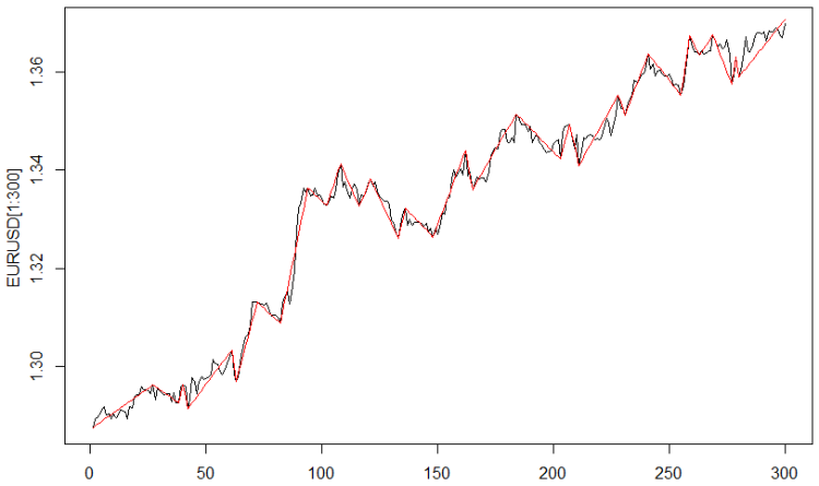
Fig. 1. The ZigZag indicator

Now, the indicator values are to be converted to a categorical value where "long" = 1 and "short" = 0. 

Result is shown on Fig. 2.

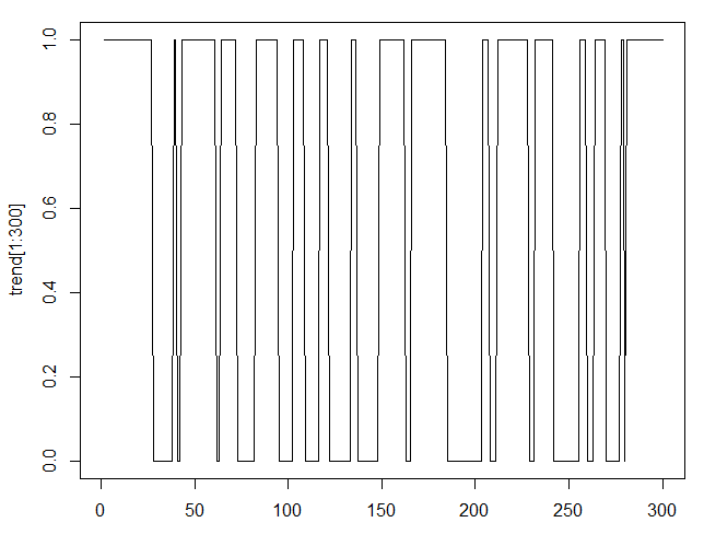
Fig. 2. The ZigZag indicator in categorical form

Let us perform the last operation with the target variable. If we shift the ZigZag indicator to the left, the current bar will correspond to the future value of the ZigZag indicator. In this article the shift is made by one bar, which is equal to a prediction of one step ahead for the data used one hour in advance.

The shift can be made for a greater number of bars and it will correlate to a prediction for a greater number of bars. This approach differs from other predictive approaches where the previous value can be used to predict several future values leading to a summation of the prediction errors.

Models highlighted in this article as well as classification models in general, do not accumulate errors. In the classification models, prediction for two bars ahead has its own prediction error not connected in any way with the prediction error for one bar ahead.

2.2. Creating Independent Variables

Independent variables or predictors are so called because they come to the model from outside. They are external, measurable variables or variables calculated based on those external variables. Any economic and financial data including quotes for currency pairs are independent variables as their values are the result of activity of market actors. Data received from technical indicators belong to the same category as they are calculated based on the quotes.

Selection of independent variables is equally as important as the choice of the target variable. In fact, it is the selection of independent variables that defines the success of modeling. The majority of the time spent on the development of the model is dedicated to analysis and selection of a set of independent variables.

Variables from the source file kot60_110101_131231_UA containing six quotes of currency pairs, time and date, can be defined as predictors.

Time and data are rather interesting from this method's perspective. There have always been attempts to use time and data in trading systems. In our models, taking into account some hidden data on the quotes dependency on the time of day and day of the week can be revealed by the classification models automatically. The only thing to do here is to convert these two variables into the categorical form. The time is to become a category with 24 levels and the date is to become a categorical variable with five levels to match the number of week days.

Besides the source predictors, we are going to create additional predictors, which, in my opinion reveal existence of trends in the source quotes. We are going to use well known indicators to create additional predictors.

The following indicators are going to be employed: 5,10 and 15; MACD(12,26,9), RSI with periods 14,21,28. On top of them we are going to use increments of quotes and moving averages. All of these conversions are to be applied to all six quotes of the currency pairs.

The ZigZag indicator will be included in the number of independent variables for supportive purposes. It is not going to be used for developing models since its value on the far right bar is unknown.

So, we have 88 independent variables, one target variable and one service variable (ZigZag). Amount of data for each of variables is 18083 bars.

This data set has the form of the R workspace and can be found in the attachment to this article with the name of TC.RData. This data set can be used as follows:

• load R;
• load the Rattle library;
• tab File/Workspace;
• find the TC.RData file on the disk and load it.

3. Intelligent Analysis of the Source Data

The Rattle package offers a set of tools for preliminary, or intelligent data processing - data mining.

3.1. Input and Preview

Let us consider some opportunities that become available after performing the actions mentioned in the section above.

The result can be seen on the picture represented on Fig. 3.

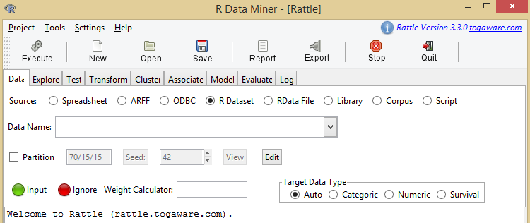
Fig. 3. Rattle home screen

Developing a model in Rattle takes place as we move from the Data tab to the Log tab.

The first tab of Rattle is Data. In accordance to its name, this tab allows loading data that can be worked with in the future.

The two buttons Spreadsheets and R Dataset are of particular interest to us.

The Spreadsheets button allows uploading Excel files. If the reader wants to test their ideas, they can prepare their own Excel file and then try out Rattle.

To repeat actions described in this article or perform some additional actions with a file containing raw data attached to this article, use the R Dataset button. This button loads the file in the R format. The file is called "Working Directory" or "Work file". They have an extension on the .RData disk. This file can be uploaded to R and it will become available by clicking this button after it.

Upload our prepared file and get the upper part of the picture on Fig. 4 and the lower part of the picture on Fig. 5.

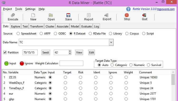
Fig. 4. Upper part of the source file

Fig. 5. Lower part of the source file

3.2. Correlation of the Target Variable with Independent Variables

Note. The "Run" button plays a crucial role. The action gets prepared but does not get performed. To carry out any action, press the "Run" button. It has to be done every time at repeating actions described in this article.

Fig. 4 shows a list of variables, their characteristics and the role of these variables. Since we are not going to use the ZigZag indicator in the models and unable to do it anyway, we will mark it as the one to ignore, i.e. set to Ignore.

Other variables are used as the input ones except for the last one, which is used as the target variable.

The Partition button plays an important role for the substantiation of the trust level to the modeling results. Using this button, the data set can be divided into three parts if required. Proportions of the data set that are used for training, validation and testing of the model are specified at this stage.

In the next field the seed for the sensor of pseudorandom numbers is specified. For example, 70% of source data gathered for the training data set is selected from the source data set randomly. As a result, the other two parts of 15% (like in our case) are also random bar sequences.

Therefore, changing Seed from the source data set, one can get an undefined amount of various training and other data sets.

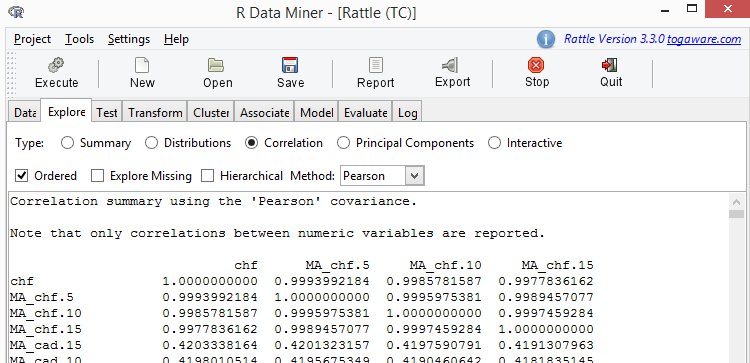
Fig. 6. Correlation of variables

Find a column with the name ZZ.35 in the received table. The sample shown in the table below was taken from that column.

Variable	ZZ.35
RSI_cad.14	-0.0104122177
JPY.dif2	-0.0088412685
EUR.dif3	-0.0052379279
CHF.dif3	-0.0049692265
GBP.dif3	-0.0047409208
GBP.dif1	0.0044691430
MA_cad.15.dif1	-0.0039004722
JPY.dif1	-0.0023831247
GBP.dif2	-0.0015356091
EUR.dif2	-0.0013759749
CHF.dif2	-0.0012447101
EUR.dif1	0.0005863149
MA_cad.10.dif1	0.0023981433
CHF.dif1	0.0024543973
MA_gbp.5.dif1	0.0043757197
MA_cad.5.dif1	0.0075424397
MA_gbp.10.dif1	0.0094964069
EURGBP.dif1	0.0095990416
CAD.dif1	0.0110571043

Table 1.  Correlation of Variables

As we can see, there is quite a long list of variables having a correlation with ZZ.35 less than 0.01. The level of correlation, less than 0.1 does not allow to come to any conclusion about the influence of independent variables on the target variable.

At this stage we are going to note this fact and use it as appropriate after the models have been assessed.

In the classification models, the degree of influence of predictors on the target variable plays a very important role. At a low correlation level, the matching predictor is believed to be the noise in the model, which leads to its retraining. Retraining of the model is when the model starts taking into account details and predictors insignificant for the target variable.

There are no recommendations on the correlation level. Usually, they use the magical number of statistics – 5%. It is incorrect in essence. Removing predictors, which are the noise in the model, leads to the reduction of the prediction error. Removing a predictor that is not the noise in the model, leads to the increase of the prediction error. Therefore the minimum list of predictors useful for the model are established through experiments.

3.3. Scaling

Some models, like support vector machines (SVM), are very sensitive to different scale of predictors, which means the following. For instance, data on the currency pair EURUSD changes within the limit of 0.5, whereas USDJPY changes within a couple of dozen units. To exclude different scale of predictors, they are to be brought to one scale in the Transform tab. It is preferable that fluctuations of predictors happen within the limit of [0-1].

To perform scaling, select Transform/Rescale/Scale [0-1]. After that we tick all variables and press the "Run" button.

3.4. Converting into the Categorical Form

Conversion into the categorical form allows converting the value of a numerical variable into a factor with several levels. The RSI indicator is the first one to be converted into a multi-level factor. It is believed to show a trend reversal when its values are approaching zero or 100.

To convert values of the RSI indicator into the categorical form, select: Transform/Recode/KMeans. Doing that, set the number of factor levels at 8. Tick all RSI indicators and press "Run".

After setting the ZZ.35 variable to Ignore then we can move on to developing models.

4. General Algorithm of the Classification Model

The following models are available in Rattle:

• model of tree-like classification (Tree);
• random forest model (forest);
• boosting trees model (ada);
• support vector machines model (SVM);
• generalized linear model (glm);
• neural network model (NNET).

Despite the fundamental difference between classification models, (we are not talking about only those available in Rattle) all of them have common features described below.

Let us take a training set consisting of strings (in our case the number is 18030), containing values of predictors (88 in our case) and the value of the target variable ("long" and "short").

Any of the classification algorithms address the problem of separating the combinations of predictor values correspondent to "long" from the combinations of predictor values correspondent to "short". This is a stage of training a model.

Then, follows the stage of verifying the model.

As we divided the source data set into three parts, we take another data set and consider combinations of predictors being compared with those received at the training stage. Every combination of predictors is established if it belongs to "short" or "long". Since the verification data set contains those known values, the result is compared with the factual data. The ratio of factual long and short positions to the predicted ones is the prediction error.

If the result does not suit us, we can return to the stage of the intelligent data analysis to improve the result. Unfortunately, the quality of this stage is completely defined by a trader's experience. Changes are made in the source data set and then a model gets developed again.

If we find the results obtained on the training and verification data sets satisfactory, then we verify the model on the test data set, that is the one that has not been used.

The model quality is defined not only by a small prediction error but also by small difference between the values of this error on different data sets. This shows robustness of the model and absence of retraining or as traders call it ultra adjustment.

In this article only a random forest model is going to be looked at in detail.

5. Random Forest Model

5.1. Summary

Algorithm of a trader's work is as follows. A set of indicators is added to a quote of a currency pair and a trade decision is made judging the total of the current quotes and indicator data.

In the simplest trading system "Moving Average", they buy if the current price is higher than the moving average and sell if it is below it. They can add additional conditions like data received from the RSI indicator. As a result, a trader gets a decision tree. In the leaves of that tree there are the quotes of the currency pair, values of the moving average and the RSI indicator. The root of the tree contains only two values - "buy" and "sell".

The described process of building a tree was automated in the model of classification trees. As a result, there is only one tree, or, in traders' slang, one pattern.

The algorithm of a single tree is unable to build precise models as diversity leads to instability, which can be seen at building separate decision trees.

A reader can verify this statement themselves using the Tree model in Rattle. This model implements the described algorithm of building a tree.

The idea of the random forest model is in including many classification trees (patterns) in the model, not just one. So, random forest tends to have higher resistance to data changes and the noise (that is variables that have little influence on the target variable).

Randomness used by the random forest algorithm is manifested in the choice both of the rows of the table (observations) and predictors. This randomness defines the significant resistance to noise, outliers and retraining when comparing with a standalone tree-like classifier.

Probability also defines significant computational efficiency. Building a standalone decision tree, the developer of the model can select a random subset of observations available in the training data set. Besides, in every node of the process of building a tree, they consider only a small part of all available variables at establishing the best proportion of splitting a data set. It leads to a significant relaxation of the requirements to the computational performance.

So, the random forest model is a good choice for developing models for a number of reasons. Very often a small preliminary data processing is required as data is not supposed to be normalized and the approach is elastic to outliers. Necessity to select variables can be avoided as the algorithm efficiently chooses own set of variables. As a lot of trees are being built using two levels of randomness (observations and predictors), every tree is an efficient independent model. This model is not prone to retraining on the training data set.

Algorithms of random forests often generate from 100 to 500 trees. When the final model is developed, the decisions made by every tree are integrated by processing the trees as equal. The final decision on an assembly of trees will be the decision on the major part of constituent trees. If 51 trees out of 100 point at "long", then the value of "long" will be accepted, though, with less confidence.

5.2. Algorithm

5.2.1. Forming a Sample from a Data Set

The algorithm of forming a random tree generates many decision trees using bootstrap aggregation or bagging for short for introducing randomness into the process of sample formation. Bootstrap aggregation is an idea of gathering a random sample of observations into a bag. Many bags formed in a random order consist of selected observations received from source observations on the training data set.

Collating to the bags is performed with substitution. It means that every observation has a chance of multiple appearances in a certain bag. The sample size is often the same as the complete data set. Practice shows that two thirds of observations will be included into a bag (with repetitions) and one third will not be taken into account. Every bag of observations is used as a training data set for building a decision tree. The unaccounted observations can be used as an independent sample to assess the result.

5.2.2. Forming the Choice of Predictors

The second basic element of randomness concerns the choice of predictors for splitting a data set. At every step of creating a separate decision node, i.e. at every splitting point of a tree, a random and usually small set of predictors is selected. Only the predictors selected at the splitting point are considered. For every node in building a tree, they consider a different random set of predictors.

5.2.3. Randomness

Forming random sets of both data and variables, they receive decision trees with various results depending on data subset. This very change allows treating this assembly of trees as a team of cooperating experts with different level of competency that make the most reliable prediction.

Sample formation also has another meaningful advantage - computation efficiency. Considering only a small part of the total number of predictors when splitting a data set significantly reduces volumes of required computations.

Creating every decision tree, the algorithm of forming a random tree usually does not cut decision trees. A random forest with ultra adjusted trees can develop a very good model, which works well on new data.

5.2.4. Calculation in the Assembly

When treating many decision trees as one model, every tree is equally important in the final decision making. Simple majority determines the result. That means that 51% of splits and 99% of splits will produce the same class, for example "long".

Calculations by Rattle are partial as the user gets the result in the form of a class. If the model is used in R, results in the form of a class probability become available.

5.3. Developing a Random Forest Model

To build a model, select Model/Forest. Started calculation of the model will take a couple of minutes for our source data.

I will divide the result of the calculation in several parts and will comment on each of them.

Let us review the results brought on Fig. 7.

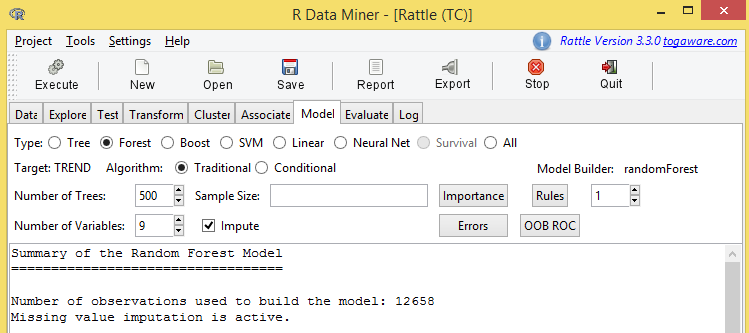
Fig. 7. The upper part of the adjustment results of the random forest model

Some information on this figure should be highlighted.

TREND is a target variable here.

500 trees were generated at building this model. At splitting in every node of the tree, 9 predictors (variables) were used. Besides, buttons Errors and OOB ROC are of special interest to us.

Then follow the prediction errors, which look like:

OOB estimate of error rate: 15.97%

Confusion matrix:

	0	1	class.error
0	4960	1163	0.1899396
1	858	5677	0.1312930

Table 2. Contingency Table of Error Matrix for the Training Set

It should be interpreted as "Error out of bag is 15.97%".

The obtained prediction error is significant. It is important to figure out how it was obtained or to be precise, if it was obtained "out of bag". Only a part of the training data set was used for developing this model. This model, in its turn, makes 70% of the source data set. Approximately 60% of the training data set was used for building this model and 40% was not used. This 40% of data is called "Out of bag". The prediction error of 15.97% was received on that data.

Moving on.

Contingency table or error matrix is interpreted the following way. 

The top row contains predicted short and long positions. The left side column is a column with actual short and long positions, received from the ZigZag indicator for historical data.

The value of 4960 with coordinates (0,0) is a number of correctly predicted short and long positions. The next value of 1163 is the number of short positions predicted as long ones.

The value of 858 with coordinates (1,0) is a number of long positions predicted as short ones. The value of 5677 is the number of correctly predicted long positions.

Then we move on to the results of modeling.

Below are a few rows of the large table comprising all variables of the model. This is a table of importance of variables.

	0	1	MeanDecreaseAccuracy	MeanDecreaseGini
MA_eur.5.dif1	42.97	41.85	54.86	321.86
EUR.dif3	37.21	46.38	51.80	177.34
RSI_eur.14	37.70	40.11	50.75	254.61
EUR.dif2	24.66	31.64	38.24	110.83
MA_eur.10.dif1	22.94	25.39	31.48	193.08
CHF.dif3	22.91	23.42	30.15	73.36
MA_chf.5.dif1	21.81	23.24	29.56	135.34

Table 3. Importance of Variables in the Random Forest Model

There are several assessments of the importance of variables. The word "importance" here reflects the degree of influence of a certain variable on the target variable. The greater the value, the more "important" the variable is.

This table provides data for excluding least significant values from the model. In statistics and in classification in particular, the simpler a model is the better, as long as the model accuracy is not sacrificed.

The Errors button is the last important thing in the Model tab. By pressing it we shall receive Fig.8.

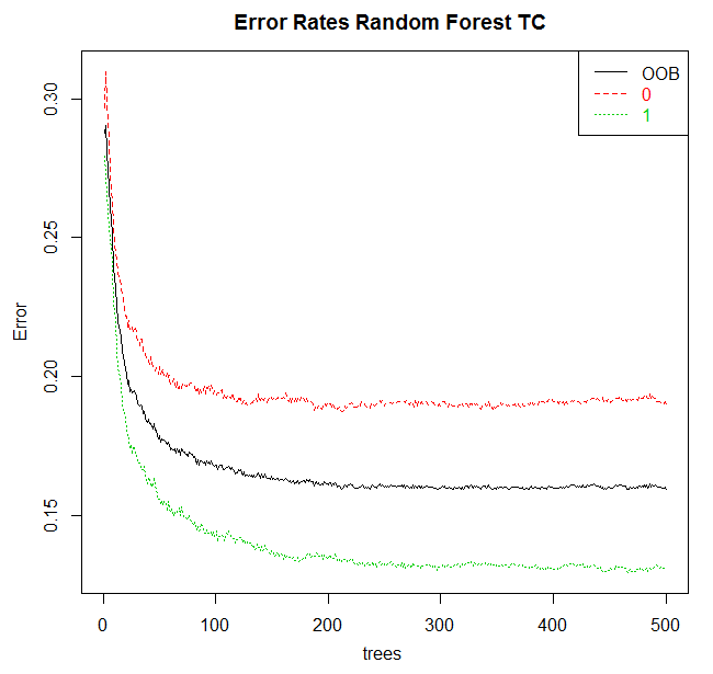
Fig. 8. Dependence of modeling error on the number of trees

6. Model Efficiency

Evaluation of the model efficiency is carried out in the Evaluate tab, where Rattle gives access to the set of options for that.

We shall use Error Matrix, as it was previously called Contingency Table, in the list of available options of model efficiency evaluation.

When you move from the Model tab to the Evaluate tab, the last of the created models will be automatically flagged. It matches the general principle of work in Rattle: we create and set up a model and then explore its efficiency in the Evaluate tab.

For the evaluation of a model, the data set for performing the check has to be specified. The next line of options in the Rattle interface is a set of alternative sources of data.

The first four options for Data correspond to splitting the data set specified in the Data tab. The options are Training, Validation, Test and Full (the whole set). Splitting data set into sets of training, validation and testing has already been discussed.

The first option is supposed to validate the model on the training data set. Usually it is not a good idea. The issue with assessing the model on the training data set is that the model was built on this data set. There the model will give a good result as it initially was what we were trying to achieve. The model is designed to be used on previously unknown data.

An approach is required to ensure good performance of the model on new data. At the same time, we obtain an actual rating of the model errors, which reflects the difference between prediction for the model and factual data. This error rating on an unknown data set, not the training one, is the best way to evaluate the model efficiency.

We use the Validation data set for verification of the model efficiency at its creation and setting up. Therefore after the model has been created, its efficiency will be verified on this verification data set. Some setting up options for creating a model can be changed. We compare the new model with the old one with its efficiency based on the verification data set. In this sense, the verification data set is used in the modeling for developing the final model. We, therefore, still have a shifted estimation of our model efficiency if we rely on the verification data set.

The Test data set is the one that was not used in creating the model at all. As soon as we identified "the best" model based on the Training and Verification data set, we can estimate the efficiency of the model on the Test data set. This is the evaluation of expected efficiency for any new data. The fourth option uses the Full data set for assessing the model. Full data set is Training, Verification and Testing data set altogether. This is nothing but curiosity and certainly not an attempt to get precise data.

Another opportunity available as data source delivered through the sample entry. It is available if the Score option is selected as the assessment type. In this case a window for entering additional data will open.

The error matrix will be used for predicting the categorical target variable.

The error matrix shows factual results against the predicted ones. There are two tables. The first one shows quantitative results and the second one shows the results in percent.

The error matrix can be found in the Evaluate tab in Rattle. Pressing "Run" will implement the selected model on the specified data set for predicting the result for every observation in this data set. Then the predictions are compared with factual observations.

Fig. 9 represents the error matrix for the random forest model calculated earlier.

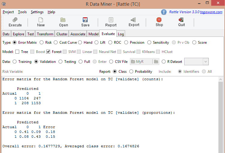
Fig. 9. Result of evaluation of the random forest model

The figure shows that the average error is 0.167, i.e. 16.7%. At the training stage prediction error was 15.97%. We can consider those values equal.

Let us perform a calculation for the Testing data set. The result is as follows:

Error matrix for the Random Forest model on TC [test] (counts):

	Predicted	Predicted
Actual	0	1
0	1016	256
1	193	1248

 Table 4. Error matrix for the random forest model in absolute terms (test data set)

Error matrix for the Random Forest model on TC [test] (proportions):

	Predicted	Predicted
Actual	0	1	Error
0	0.37	0.09	0.20
1	0.07	0.46	0.13

Table 5. Error matrix for the random forest model in relative terms (Test data set)

Overall error: 0.1654994, Averaged class error: 0.1649244

Prediction error is 16.4%.

All three figures are approximately equal, which is a sign of a reasonable result of modeling.

Please note that the efficiency of models calculated by Rattle must be checked in the Strategy Tester of МetaТrader 4 or MetaTrader 5. Then it should be tested on a demo-account and real account with small lots. Only after all test runs we can come to final conclusions about the model.

7. Improving the Model

When we explored correlation of pseudo variable ZZ.35 with predictors, we found out that a significant number of predictors had a weak correlation with the target variable.

Let us delete the predictors that have the correlation coefficient of less than 0.01. To do that, set the relevant predictors to Ignore in the Data tab and repeat calculation of the random forest model in the Model tab.

We get the following result:

• prediction error out of bag = 15.77%;
• prediction error for the Validation data set = 15.67%;
• prediction error for the Test data set = 15.77%.

Though the error reduced insignificantly, the gap between prediction errors for different data set has decreased. It is a sign of the model stability.

You can keep removing predictors following the correlation table. The model effectiveness can be improved, i.e. the prediction error decreased, using data from the table of importance of predictors that was obtained in calculating the model.

In any case, removing predictors can be done till removing of another predictor leads to deterioration of the model efficiency. You can stop at that point as you have a minimal and most efficient model for a given number of predictors.

8. Using the Model in MetaTrader 4

In theory, trading using Rattle can be organized the following way. The input data for Rattle in Excel are getting prepared by some outside tools for the period of day and night. Upon closing of the exchange, a trader gets the required prices and puts them into the source file. A few minutes later the forecast for the following day is ready and can be used straight from the opening.

The МetaТrader 4 terminal or its analogue is necessary for the intraday trading.

To organize an automated or semi-automated trading using Rattle, the following constituents are required:

• a previously trained model, which was saved as the R workspace;
• a library of cooperation of the terminal and R;
• code in R, which passes on every new block of data to the model, gets the result and sends the result of modeling back to the terminal.

Training one of the six models available in Rattle was considered above. The number of classification models available in R is coming up to 150 but Rattle is of no use for them.

The library of interaction of R and the МetaТrader 4 terminal can be found in the CodeBase: mt4R for new MQL4.

Code in R, which corresponds to the trained model is in the journal (the Log tab). All actions taken at the model development get registered in the form of code in R. This is what is to be used in real trading.

Conclusion

Both novice and experienced traders will find this article useful for preliminary evaluation and selection of a trading system.

Using Rattle, the main intellectual challenge in developing a trading system is the right choice of the target variable and predictors necessary for it. Experienced traders already have knowledge in this sphere and novices will have necessary practice with Rattle.