#
n = 100
g = 6
set.seed(g)
d <- data.frame(x = unlist(lapply(1:g, function(i) rnorm(n/g, runif(1)*i^2))),
y = unlist(lapply(1:g, function(i) rnorm(n/g, runif(1)*i^2))))
plot(d)
--------------------------------------
#1
library(fpc)
pamk.best <- pamk(d)
cat("number of clusters estimated by optimum average silhouette width:", strpamk.best$nc, "\n")
plot(pam(d, pamk.best$nc))
#2 we could also do:
library(fpc)
asw <- numeric(20)
for (k in 2:20)
asw[[k]] <- pam(d, k) $ silinfo $ avg.width
k.best <- which.max(asw)
cat("silhouette-optimal number of clusters:", k.best, "\n")
---------------------------------------------------
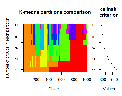
#3. Calinsky criterion: Another approach to diagnosing how many clusters suit the data. In this case
# we try 1 to 10 groups.
require(vegan)
fit <- cascadeKM(scale(d, center = TRUE, scale = TRUE), 1, 10, iter = 1000)
plot(fit, sortg = TRUE, grpmts.plot = TRUE)
calinski.best <- as.numeric(which.max(fit$results[2,]))
cat("Calinski criterion optimal number of clusters:", calinski.best, "\n")
# 5 clusters!
-------------------
4. Determine the optimal model and number of clusters according to the Bayesian Information
Criterion for expectation-maximization, initialized by hierarchical clustering for parameterized
Gaussian mixture models
library(mclust)
# Run the function to see how many clusters
# it finds to be optimal, set it to search for
# at least 1 model and up 20.
d_clust <- Mclust(as.matrix(d), G=1:20)
m.best <- dim(d_clust$z)[2]
cat("model-based optimal number of clusters:", m.best, "\n")
# 4 clusters
plot(d_clust)
----------------------------------------------------------------
5. Affinity propagation (AP) clustering, see http://dx.doi.org/10.1126/science.1136800
library(apcluster)
d.apclus <- apcluster(negDistMat(r=2), d)
cat("affinity propogation optimal number of clusters:", length(d.apclus@clusters), "\n")
# 4
heatmap(d.apclus)
plot(d.apclus, d)
---------------------------------------------------------------------
6. Gap Statistic for Estimating the Number of Clusters.
See also some code for a nice graphical
output . Trying 2-10 clusters here:
library(cluster)
clusGap(d, kmeans, 10, B = 100, verbose = interactive())
-----------------------------------------------------------------------
7. You may also find it useful to explore your data with clustergrams to visualize cluster
assignment, see http://www.r-statistics.com/2010/06/clustergram-visualization-and-diagnostics-for-cluster-analysis-r-code/
for more details.
-------------------------------------------------------------------
#8. The NbClust package provides 30 indices to determine the number of clusters in a dataset.
library(NbClust)
nb <- NbClust(d, diss = NULL, distance = "euclidean",
min.nc=2, max.nc=15, method = "kmeans",
index = "alllong", alphaBeale = 0.1)
hist(nb$Best.nc[1,], breaks = max(na.omit(nb$Best.nc[1,])))
# Looks like 3 is the most frequently determined number of clusters
# and curiously, four clusters is not in the output at all!
-----------------------------------------
Here are a few examples:
d_dist <- dist(as.matrix(d)) # find distance matrix
plot(hclust(d_dist)) # apply hirarchical clustering and plot
----------------------------------------------------
#9 Bayesian clustering method, good for high-dimension data, more details:
# http://vahid.probstat.ca/paper/2012-bclust.pdf
install.packages("bclust")
library(bclust)
x <- as.matrix(d)
d.bclus <- bclust(x, transformed.par = c(0, -50, log(16), 0, 0, 0))
viplot(imp(d.bclus)$var);
plot(d.bclus);
ditplot(d.bclus)
dptplot(d.bclus, scale = 20, horizbar.plot = TRUE,varimp = imp(d.bclus)$var, horizbar.distance = 0, dendrogram.lwd = 2)
-------------------------------------------------------------------------
#10 Also for high-dimension data is the pvclust library which calculates
#p-values for hierarchical clustering via multiscale bootstrap resampling. Here's #the example from the documentation (wont work on such low dimensional data as in #my example):
library(pvclust)
library(MASS)
data(Boston)
boston.pv <- pvclust(Boston)
plot(boston.pv)
------------------------------------
###Automatically cut the dendrogram
require(dynamicTreeCut)
ct_issues <- cutreeHybrid(hc_issues, inverse_cc_combined, minClusterSize=5)
-----
FANNY <- fanny(as.dist(inverse_cc_combined),, k = 3, maxit = 2000)
FANNY$membership MDS <- smacofSym(distMat)$conf
plot(MDS, type = "n") text(MDS, label = rownames(MDS), col = rgb((FANNY$membership)^(1/1)))
-----
m7 <- stepFlexmix
----------------------
#11 "clusterSim" -Department of Econometrics and Computer Science, University of #Economics, Wroclaw, Poland
http://keii.ue.wroc.pl/clusterSim
See file ../doc/clusterSim_details.pdf for further details
data.Normalization Types of variable (column) and object (row) normalization formulas
Description
Types of variable (column) and object (row) normalization formulas
Usage
data.Normalization (x,type="n0",normalization="column")
Arguments
x vector, matrix or dataset
type type of normalization: n0 - without normalization
n1 - standardization ((x-mean)/sd)
n2 - positional standardization ((x-median)/mad)
n3 - unitization ((x-mean)/range)
n3a - positional unitization ((x-median)/range)
n4 - unitization with zero minimum ((x-min)/range)
n5 - normalization in range <-1,1> ((x-mean)/max(abs(x-mean)))
n5a - positional normalization in range <-1,1> ((x-median)/max(abs(x-median)))
n6 - quotient transformation (x/sd)
n6a - positional quotient transformation (x/mad)
n7 - quotient transformation (x/range)
n8 - quotient transformation (x/max)
n9 - quotient transformation (x/mean)
n9a - positional quotient transformation (x/median)
n10 - quotient transformation (x/sum)
n11 - quotient transformation (x/sqrt(SSQ))
normalization "column" - normalization by variable, "row" - normalization by objec
See file ../doc/HINoVMod_details.pdf for further details
> library(fpc)
> pamk.best <- pamk(x)
> cat("number of clusters estimated by optimum average silhouette width:", pamk.best$nc, "\n")
> number of clusters estimated by optimum average silhouette width: h: 2
> require(vegan)
> fit <- cascadeKM(scale(x, center = TRUE,  scale = TRUE), 1, 10, iter = 1000)
> plot(fit, sortg = TRUE, grpmts.plot = TRUE)
> calinski.best <- as.numeric(which.max(fit$results[2,]))
> cat("Calinski criterion optimal number of clusters:", calinski.best, "\n")
Calinski criterion optimal number of clusters: 2
> library(mclust)
# Run the function to see how many clusters
# it finds to be optimal, set it to search for# at least 1 model and up 20.
> d_clust <- Mclust(as.matrix(x), G=1:20)
> m.best <- dim(d_clust$z)[2]
> cat("model-based optimal number of clusters:", m.best, "\n")
model-based optimal number of clusters: 7
私への質問ではない。記事について言いたいことはそれだけですか?
記事については?典型的なリライトだ。他の情報源でも同じことで、言葉が少し違うだけ。写真も同じ。新しいもの、つまり著者らしいものは何も見当たりませんでした。
例を試してみたかったのだが、残念だ。このセクションはMQL5用だが、例題はMQL4用だ。
vlad1949
親愛なるVlad!
アーカイブを見ましたが、Rのドキュメントがかなり古いですね。添付のコピーに変更するのが良いでしょう。
vlad1949
ヴラドへ
なぜテスターで失敗したのですか?
私はすべて問題なく動作しています。しかし、スキームはインジケータなしです:Expert AdvisorはRと直接通信します。
ディープネットワークの発明者、ジェフリー・ヒントン:「ディープネットワークは、信号対雑音比が大きいデータにしか適用できない。金融系列はノイズが多いので、ディープネットワークは適用できない。試してみたがダメだった"
YouTubeで彼の講義を聴く。
ディープネットワークの発明者、ジェフリー・ヒントン:「ディープネットワークは、信号対雑音比が大きいデータにしか適用できない。金融系列はノイズが多いので、ディープネットワークは適用できない。試してみたがダメだった"
ユーチューブで彼の講義を聞いてみよう。
並行スレッドでのあなたの投稿を考慮すると。
ノイズは、分類タスクと無線工学では異なって理解される。予測変数がノイズとみなされるのは、それがターゲット変数に対して弱い関連性を持つ(予測力が弱い)場合である。全く異なる意味です。ターゲット変数の異なるクラスに対して予測力を持つ予測変数を探すべきです。
私はノイズについても同様の理解を持っている。金融系列は多くの予測変数に依存しており、そのほとんどが未知のもので、この「ノイズ」を系列に導入している。公開されている予測変数のみを使用すると、どのようなネットワークや方法を使用しても、ターゲット変数を予測することはできません。
vlad1949
ヴラドへ
なぜテスターで失敗したのですか?
私はすべて問題なく動作しています。インジケータのないスキームを真にします:アドバイザーは直接Rと通信します。
llllllllllllllllllllllllllllllllllllllllllllllllllllllllllllllllllllllllllllllllllllllllllllllllllllllllll
こんにちは、SanSanychです。
つまり、主なアイデアは、いくつかの指標でマルチ通貨を作ることです。
そうでなければ、もちろん、Expert Advisorにすべてを詰め込むことができます。
しかし、トレーニング、テスト、最適化を、取引を中断することなく、その場で 実行するので あれば、1つのExpert Advisorを使用したバリアントを実装するのは少し難しくなります。
幸運を祈る。
PS.テストの結果は?
SanSanychさん、こんにちは。
英語圏のフォーラムで見つけた、最適なクラスター数を決定する例をいくつか紹介します。私のデータでは、これらすべてを使用することはできませんでした。clusterSim " パッケージはとても興味深いです。
--------------------------------------------------------------------------------------
次の投稿では、私のデータを使って計算します
最適なクラスター数は、いくつかのパッケージによって、30以上の最適化基準を用いて決定することができる。私の観察によると、最も使われている基準は Calinsky基準 である。
インジケータ dt のセットから生データを取り出しましょう 。これには17の予測変数、ターゲットy、ローソク足本体zが含まれています。
最新バージョンの "magrittr " と "dplyr " パッケージには多くの新機能が あります 。 これは中間結果を保存する必要がない場合に非常に便利である。クラスタリングのための初期データを準備しよう。初期行列dtを取り、そこから最後の1000行を選択し、そこから変数の17列を選択します。より明確な表記が得られますが、それ以上のことはありません。
1.
2.Calinsky基準:データにいくつのクラスタが適しているかを診断するもう1つのアプローチ。この場合
1~10のグループを試す。
3.パラメータ化ガウス混合モデルの階層クラスタリングによって初期化された、期待値最大化のためのベイズ情報量基準に従って、最適モデルとクラスタ数を決定する。ガウス混合モデル