Principles of batch normalization implementation
The authors of the method proposed the following normalization algorithm. First, we calculate the average value from the data sample.
where:
- μB = arithmetic mean of the dataset
- m = dataset size (batch)
Then we calculate the variance of the initial sample.
Next, we will normalize the dataset by making it have a zero mean and a unit variance.
Please note that a small positive number ε is added to the denominator of the dataset variance to avoid division by zero.
However, it has been found that such normalization can distort the impact of the initial data. Therefore, the authors of the method added another step that includes scaling and shifting. They introduced variables γ and β, which are trained along with the neural network using gradient descent.
The application of this method allows obtaining a dataset with the same distribution at each training step, which, in practice, makes neural network training more stable and enables an increase in the learning rate. Overall, this can improve the training quality while reducing the time and computational resources required for neural network training.
However, at the same time, the costs of storing additional coefficients increase. Additionally, the calculation of moving averages and variances requires additional memory allocation to store historical data for each neuron across the entire batch size. Here you can look at the exponential average. To calculate EMA (Exponential Moving Averages), we only need the previous value of the function and the current element of the sequence.
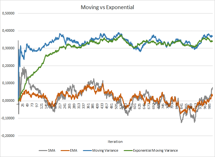
The figure below provides a visual comparison of moving averages and moving variances for 100 elements against exponential moving averages and exponential moving variances for the same 100 elements. The graph was plotted for 1,000 random items in the range from -1.0 to 1.0.

Comparison of moving and exponential average graphs
As seen in the graph, the moving average and exponential moving average converge after around 120-130 iterations, and beyond that point, there is minimal deviation that can be disregarded. The exponential moving average chart also looks smoother. To calculate EMA, you only need the previous value of the function and the current element of the sequence. Let me remind you of the exponential moving average formula.
where:
- μi = exponential average of the sample at the ith step
- m = dataset size (batch)
- xi = current value of the indicator
To align the plots of moving variance and exponential moving variance, it took slightly more iterations (around 310-320), but overall the picture is similar. In the case of variance, the use of exponential moving averages not only saves memory but also significantly reduces the number of computations since for moving variance, we would need to recalculate the deviation from the mean for the entire batch of historical data, which can be computationally expensive.
In my opinion, the use of such a solution significantly reduces memory usage and the computational overhead during each iteration of the forward pass.