저도 노이즈에 대해 비슷한 이해를 가지고 있습니다. 재무 계열은 수많은 예측 변수에 의존하며, 그 중 대부분은 우리가 알 수 없고 이러한 '노이즈'를 계열에 도입합니다. 공개적으로 사용 가능한 예측 변수만 사용하면 어떤 네트워크나 방법을 사용하든 목표 변수를 예측할 수 없습니다.
gpwr: 저도 노이즈에 대해 비슷한 이해를 가지고 있습니다. 금융 계열은 수많은 예측 변수에 의존하는데, 그 중 대부분은 우리에게 알려지지 않았고 이러한 '노이즈'를 계열에 도입합니다. 공개적으로 사용 가능한 예측 변수만 사용하면 어떤 네트워크나 방법을 사용하든 대상 변수를 예측할 수 없습니다.
#
n = 100
g = 6
set.seed(g)
d <- data.frame(x = unlist(lapply(1:g, function(i) rnorm(n/g, runif(1)*i^2))),
y = unlist(lapply(1:g, function(i) rnorm(n/g, runif(1)*i^2))))
plot(d)
--------------------------------------
#1
library(fpc)
pamk.best <- pamk(d)
cat("number of clusters estimated by optimum average silhouette width:", strpamk.best$nc, "\n")
plot(pam(d, pamk.best$nc))
#2 we could also do:
library(fpc)
asw <- numeric(20)
for (k in 2:20)
asw[[k]] <- pam(d, k) $ silinfo $ avg.width
k.best <- which.max(asw)
cat("silhouette-optimal number of clusters:", k.best, "\n")
---------------------------------------------------
#3. Calinsky criterion: Another approach to diagnosing how many clusters suit the data. In this case
# we try 1 to 10 groups.
require(vegan)
fit <- cascadeKM(scale(d, center = TRUE, scale = TRUE), 1, 10, iter = 1000)
plot(fit, sortg = TRUE, grpmts.plot = TRUE)
calinski.best <- as.numeric(which.max(fit$results[2,]))
cat("Calinski criterion optimal number of clusters:", calinski.best, "\n")
# 5 clusters!
-------------------
4. Determine the optimal model and number of clusters according to the Bayesian Information
Criterion for expectation-maximization, initialized by hierarchical clustering for parameterized
Gaussian mixture models
library(mclust)
# Run the function to see how many clusters
# it finds to be optimal, set it to search for
# at least 1 model and up 20.
d_clust <- Mclust(as.matrix(d), G=1:20)
m.best <- dim(d_clust$z)[2]
cat("model-based optimal number of clusters:", m.best, "\n")
# 4 clusters
plot(d_clust)
----------------------------------------------------------------
5. Affinity propagation (AP) clustering, see http://dx.doi.org/10.1126/science.1136800
library(apcluster)
d.apclus <- apcluster(negDistMat(r=2), d)
cat("affinity propogation optimal number of clusters:", length(d.apclus@clusters), "\n")
# 4
heatmap(d.apclus)
plot(d.apclus, d)
---------------------------------------------------------------------
6. Gap Statistic for Estimating the Number of Clusters.
See also some code for a nice graphical
output . Trying 2-10 clusters here:
library(cluster)
clusGap(d, kmeans, 10, B = 100, verbose = interactive())
-----------------------------------------------------------------------
7. You may also find it useful to explore your data with clustergrams to visualize cluster
assignment, see http://www.r-statistics.com/2010/06/clustergram-visualization-and-diagnostics-for-cluster-analysis-r-code/
for more details.
-------------------------------------------------------------------
#8. The NbClust package provides 30 indices to determine the number of clusters in a dataset.
library(NbClust)
nb <- NbClust(d, diss = NULL, distance = "euclidean",
min.nc=2, max.nc=15, method = "kmeans",
index = "alllong", alphaBeale = 0.1)
hist(nb$Best.nc[1,], breaks = max(na.omit(nb$Best.nc[1,])))
# Looks like 3 is the most frequently determined number of clusters
# and curiously, four clusters is not in the output at all!
-----------------------------------------
Here are a few examples:
d_dist <- dist(as.matrix(d)) # find distance matrix
plot(hclust(d_dist)) # apply hirarchical clustering and plot
----------------------------------------------------
#9 Bayesian clustering method, good for high-dimension data, more details:
# http://vahid.probstat.ca/paper/2012-bclust.pdf
install.packages("bclust")
library(bclust)
x <- as.matrix(d)
d.bclus <- bclust(x, transformed.par = c(0, -50, log(16), 0, 0, 0))
viplot(imp(d.bclus)$var);
plot(d.bclus);
ditplot(d.bclus)
dptplot(d.bclus, scale = 20, horizbar.plot = TRUE,varimp = imp(d.bclus)$var, horizbar.distance = 0, dendrogram.lwd = 2)
-------------------------------------------------------------------------
#10 Also for high-dimension data is the pvclust library which calculates
#p-values for hierarchical clustering via multiscale bootstrap resampling. Here's #the example from the documentation (wont work on such low dimensional data as in #my example):
library(pvclust)
library(MASS)
data(Boston)
boston.pv <- pvclust(Boston)
plot(boston.pv)
------------------------------------
###Automatically cut the dendrogram
require(dynamicTreeCut)
ct_issues <- cutreeHybrid(hc_issues, inverse_cc_combined, minClusterSize=5)
-----
FANNY <- fanny(as.dist(inverse_cc_combined),, k = 3, maxit = 2000)
FANNY$membership MDS <- smacofSym(distMat)$conf
plot(MDS, type = "n") text(MDS, label = rownames(MDS), col = rgb((FANNY$membership)^(1/1)))
-----
m7 <- stepFlexmix
----------------------
#11 "clusterSim" -Department of Econometrics and Computer Science, University of #Economics, Wroclaw, Poland
http://keii.ue.wroc.pl/clusterSim
See file ../doc/clusterSim_details.pdf for further details
data.Normalization Types of variable (column) and object (row) normalization formulas
Description
Types of variable (column) and object (row) normalization formulas
Usage
data.Normalization (x,type="n0",normalization="column")
Arguments
x vector, matrix or dataset
type type of normalization: n0 - without normalization
n1 - standardization ((x-mean)/sd)
n2 - positional standardization ((x-median)/mad)
n3 - unitization ((x-mean)/range)
n3a - positional unitization ((x-median)/range)
n4 - unitization with zero minimum ((x-min)/range)
n5 - normalization in range <-1,1> ((x-mean)/max(abs(x-mean)))
n5a - positional normalization in range <-1,1> ((x-median)/max(abs(x-median)))
n6 - quotient transformation (x/sd)
n6a - positional quotient transformation (x/mad)
n7 - quotient transformation (x/range)
n8 - quotient transformation (x/max)
n9 - quotient transformation (x/mean)
n9a - positional quotient transformation (x/median)
n10 - quotient transformation (x/sum)
n11 - quotient transformation (x/sqrt(SSQ))
normalization "column" - normalization by variable, "row" - normalization by objec
See file ../doc/HINoVMod_details.pdf for further details
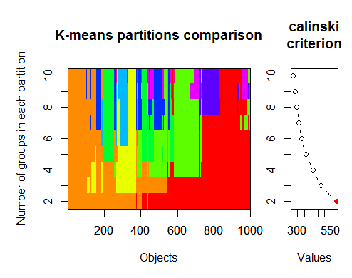
최적의 클러스터 수는 여러 패키지와 30개 이상의 최적성 기준을 사용하여 결정할 수 있습니다. 제가 관찰한 바에 따르면 가장 많이 사용되는 기준은 칼린스키 기준입니다 .
지표 dt 에서 세트의 원시 데이터를 가져와 보겠습니다 . 여기에는 17개의 예측 변수, 목표 Y 및 캔들 몸통 Z가 포함되어 있습니다.
최신 버전의 "magrittr" 및 "dplyr"패키지에는 새롭고 멋진 기능이 많이 있는데, 그중 하나가 '파이프' - %>%입니다. 중간 결과를 저장할 필요가 없을 때 매우 편리합니다. 클러스터링을 위한 초기 데이터를 준비해 보겠습니다. 초기 행렬 dt를 가져와서 마지막 1000개의 행을 선택한 다음 이 행렬에서 변수의 17개 열을 선택합니다. 더 명확한 표기법을 얻을 수 있습니다.
> library(fpc)
> pamk.best <- pamk(x)
> cat("number of clusters estimated by optimum average silhouette width:", pamk.best$nc, "\n")
> number of clusters estimated by optimum average silhouette width: h: 2
2. 칼린스키 기준: 데이터에 얼마나 많은 클러스터가 적합한지 진단하는 또 다른 접근 방식입니다. 이 경우
1~10개의 그룹을 시도합니다.
> require(vegan)
> fit <- cascadeKM(scale(x, center = TRUE,  scale = TRUE), 1, 10, iter = 1000)
> plot(fit, sortg = TRUE, grpmts.plot = TRUE)
> calinski.best <- as.numeric(which.max(fit$results[2,]))
> cat("Calinski criterion optimal number of clusters:", calinski.best, "\n")
Calinski criterion optimal number of clusters: 2
3. 매개변수화된 가우스 혼합 모델에 대해 계층적 클러스터링으로 초기화된 기대 최대화를 위한 베이지안 정보 기준에 따라 최적의 모델과 클러스터 수를 결정합니다.
가우스 혼합 모델
> library(mclust)
# Run the function to see how many clusters
# it finds to be optimal, set it to search for# at least 1 model and up 20.
> d_clust <- Mclust(as.matrix(x), G=1:20)
> m.best <- dim(d_clust$z)[2]
> cat("model-based optimal number of clusters:", m.best, "\n")
model-based optimal number of clusters: 7
저에게는 질문이 아닙니다. 기사에 대해 할 말이 그게 다인가요?
기사는 어때요? 전형적인 재작성입니다. 단어만 약간 다를 뿐 다른 출처에서도 똑같은 내용입니다. 심지어 사진도 똑같아요. 새로운 내용, 즉 저자의 독창성이 느껴지지 않았어요.
예제를 사용해보고 싶었지만 아쉽습니다. 섹션은 MQL5용이지만 예제는 MQL4용입니다.
vlad1949
친애하는 블라드!
아카이브를 살펴보니 다소 오래된 R 문서가 있습니다. 첨부된 사본으로 변경하는 것이 좋을 것 같습니다.
vlad1949
블라드에게!
왜 테스터에서 실행하지 못했나요?
나는 모든 것이 문제없이 작동합니다. 그러나이 계획에는 지표가 없습니다. 전문가 고문은 R과 직접 통신합니다.
딥 네트워크의 발명가 Jeffrey Hinton: "딥 네트워크는 신호 대 잡음비가 큰 데이터에만 적용할 수 있습니다. 금융 계열은 노이즈가 너무 커서 딥 네트워크를 적용할 수 없습니다. 우리는 시도해 보았지만 운이 없었습니다."
YouTube에서 그의 강연을 들어보세요.
딥 네트워크의 발명가 Jeffrey Hinton: "딥 네트워크는 신호 대 잡음비가 큰 데이터에만 적용할 수 있습니다. 금융 계열은 노이즈가 너무 커서 딥 네트워크를 적용할 수 없습니다. 우리는 시도해봤지만 운이 없었습니다."
유튜브에서 그의 강의를 들어보세요.
병렬 스레드에서 게시물을 고려합니다.
분류 작업에서 노이즈는 무선 공학에서와는 다르게 이해됩니다. 예측 변수가 대상 변수와 관련성이 약하면(예측력이 약하면) 노이즈가 있는 것으로 간주합니다. 완전히 다른 의미입니다. 대상 변수의 다양한 클래스에 대해 예측력이 있는 예측자를 찾아야 합니다.
저도 노이즈에 대해 비슷한 이해를 가지고 있습니다. 금융 계열은 수많은 예측 변수에 의존하는데, 그 중 대부분은 우리에게 알려지지 않았고 이러한 '노이즈'를 계열에 도입합니다. 공개적으로 사용 가능한 예측 변수만 사용하면 어떤 네트워크나 방법을 사용하든 대상 변수를 예측할 수 없습니다.
vlad1949
블라드에게!
왜 테스터에서 실행하지 못했나요?
나는 모든 것이 문제없이 작동합니다. 표시기가없는 계획 : 고문이 R과 직접 통신합니다.
ㅋㅋㅋㅋ ㅋㅋㅋㅋ ㅋㅋㅋㅋ ㅋㅋㅋㅋ ㅋㅋㅋㅋ ㅋㅋㅋㅋ ㅋㅋㅋㅋ ㅋㅋㅋㅋ ㅋㅋㅋㅋ ㅋㅋㅋㅋ ㅋㅋㅋㅋ ㅋㅋㅋㅋ ㅋㅋㅋㅋ ㅋㅋㅋㅋ ㅋㅋㅋㅋ ㅋㅋㅋㅋ ㅋㅋㅋㅋ ㅋㅋㅋㅋ ㅋㅋㅋㅋ ㅋㅋㅋㅋ ㅋㅋㅋㅋ ㅋㅋㅋㅋ ㅋㅋㅋㅋ ㅋㅋㅋㅋ ㅋㅋㅋㅋ ㅋㅋㅋㅋ ㅋㅋㅋㅋ ㅋㅋㅋㅋ ㅋㅋㅋㅋㅋㅋ
안녕하세요 산산치입니다.
따라서 주요 아이디어는 여러 지표로 다중 통화를 만드는 것입니다.
물론 그렇지 않으면 모든 것을 전문가 어드바이저에 담을 수 있습니다.
그러나 트레이딩, 테스트 및 최적화가 거래를 중단하지 않고 즉석에서 구현된다면 전문가 어드바이저가 하나 인 변형은 구현하기가 조금 더 어려울 것입니다.
행운을 빕니다.
추신 테스트 결과는 어떤가요?
안녕하세요 산산치입니다.
다음은 영어권 포럼에서 찾은 최적의 클러스터 수를 결정하는 몇 가지 예입니다. 내 데이터로 모두 사용할 수 없었습니다. 매우 흥미로운 11 패키지 "clusterSim".
--------------------------------------------------------------------------------------
다음 포스트에서 내 데이터로 계산
최적의 클러스터 수는 여러 패키지와 30개 이상의 최적성 기준을 사용하여 결정할 수 있습니다. 제가 관찰한 바에 따르면 가장 많이 사용되는 기준은 칼린스키 기준입니다 .
지표 dt 에서 세트의 원시 데이터를 가져와 보겠습니다 . 여기에는 17개의 예측 변수, 목표 Y 및 캔들 몸통 Z가 포함되어 있습니다.
최신 버전의 "magrittr " 및 "dplyr" 패키지에는 새롭고 멋진 기능이 많이 있는데, 그중 하나가 '파이프' - %>%입니다. 중간 결과를 저장할 필요가 없을 때 매우 편리합니다. 클러스터링을 위한 초기 데이터를 준비해 보겠습니다. 초기 행렬 dt를 가져와서 마지막 1000개의 행을 선택한 다음 이 행렬에서 변수의 17개 열을 선택합니다. 더 명확한 표기법을 얻을 수 있습니다.
1.
2. 칼린스키 기준: 데이터에 얼마나 많은 클러스터가 적합한지 진단하는 또 다른 접근 방식입니다. 이 경우
1~10개의 그룹을 시도합니다.
3. 매개변수화된 가우스 혼합 모델에 대해 계층적 클러스터링으로 초기화된 기대 최대화를 위한 베이지안 정보 기준에 따라 최적의 모델과 클러스터 수를 결정합니다.가우스 혼합 모델