4.Building a test recurrent model in Python

To build test recurrent models in Python, we will use the previously developed template. Moreover, we will take the script file convolution.py, which we used when testing convolutional models. Let's make a copy of it with the file name lstm.py. In the created copy, we leave the perceptron model and the best convolutional model, deleting the rest. This approach will allow us to compare the performance of the new models with the architectural solutions discussed earlier.

# Creating a perceptron model with three hidden layers and regularization
model1 = keras.Sequential([keras.Input(shape=inputs),
                           keras.layers.Dense(40, activation=tf.nn.swish,
                 kernel_regularizer=keras.regularizers.l1_l2(l1=1e-7, l2=1e-5)),
                           keras.layers.Dense(40, activation=tf.nn.swish,
                 kernel_regularizer=keras.regularizers.l1_l2(l1=1e-7, l2=1e-5)),
                           keras.layers.Dense(40, activation=tf.nn.swish,
                 kernel_regularizer=keras.regularizers.l1_l2(l1=1e-7, l2=1e-5)),
                           keras.layers.Dense(targerts, activation=tf.nn.tanh)
                         ])

# Model with 2-dimensional convolutional layer
model3 = keras.Sequential([keras.Input(shape=inputs),
                           # Reformat the tensor to 4-dimensional.
   # Specify 3 dimensions, because the 4th dimension is determined by the size of the packet
                           keras.layers.Reshape((-1,4,1)),
                           # Convolutional layer with 8 filters
                           keras.layers.Conv2D(8,(3,1),1,activation=tf.nn.swish,
                 kernel_regularizer=keras.regularizers.l1_l2(l1=1e-7, l2=1e-5)),
                           # Pooling layer
                           keras.layers.MaxPooling2D((2,1),strides=1),
                 # Reformat the tensor to 2-dimensional for fully connected layers
                           keras.layers.Flatten(),
                           keras.layers.Dense(40, activation=tf.nn.swish,
                 kernel_regularizer=keras.regularizers.l1_l2(l1=1e-7, l2=1e-5)),
                           keras.layers.Dense(40, activation=tf.nn.swish,
                 kernel_regularizer=keras.regularizers.l1_l2(l1=1e-7, l2=1e-5)),
                           keras.layers.Dense(40, activation=tf.nn.swish,
                 kernel_regularizer=keras.regularizers.l1_l2(l1=1e-7, l2=1e-5)),
                           keras.layers.Dense(targerts, activation=tf.nn.tanh)
                         ])

After that, we will create three new models using the recurrent LSTM block. Initially, we will take the convolutional neural network model and replace the convolutional and pooling layers with a single recurrent layer with 40 neurons at the output. Note that the input to the recurrent LSTM block should be a three-dimensional tensor of the format [batch, timesteps, feature]. Just like in the case of a convolutional layer, when specifying the dimensionality of a layer in the model, we don't explicitly mention the batch dimension, as its value is determined by the batch size of the input data.

# Add an LSTM block to the model
model2 = keras.Sequential([keras.Input(shape=inputs),
# Reformat the tensor to 3-dimensional.
# Specify 2 dimensions, because. The 3rd dimension is determined by the size of the packet
                           keras.layers.Reshape((-1,4)),
# The LSTM block contains 40 elements and returns the result at each step
                           keras.layers.LSTM(40, return_sequences=False,
                 kernel_regularizer=keras.regularizers.l1_l2(l1=1e-7, l2=1e-5)),

In this model, we specified parameter return_sequences=False which instructs the recurrent layer to produce the result only after processing the full batch. In this version, our LSTM layer returns a two-dimensional tensor in the format [batch, feature]. In this case, the dimension of the feature measurement will be equal to the number of neurons that we specified during the creation of the recurrent layer. A tensor of the same dimension is required for the input of a fully connected neural layer. Therefore, we do not need additional reformatting of the data, and we can use a fully connected neural layer.

                           keras.layers.Dense(40, activation=tf.nn.swish,
                 kernel_regularizer=keras.regularizers.l1_l2(l1=1e-7, l2=1e-5)),
                           keras.layers.Dense(40, activation=tf.nn.swish,
                 kernel_regularizer=keras.regularizers.l1_l2(l1=1e-7, l2=1e-5)),
                           keras.layers.Dense(40, activation=tf.nn.swish,
                 kernel_regularizer=keras.regularizers.l1_l2(l1=1e-7, l2=1e-5)),
                           keras.layers.Dense(targerts, activation=tf.nn.tanh)
                         ])

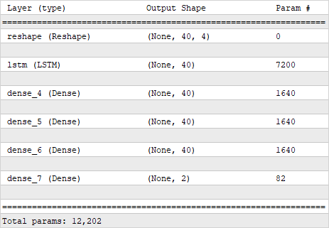
Structure of a recurrent model with four fully connected layers

In this implementation, we use the recurrent layer for preliminary data processing, while decision-making in the model is carried out by several fully connected perceptron layers that follow the recurrent layer. As a result, we got a model with 12,202 parameters.

We will compile all neural models with the same parameters. We use the Adam method for optimization and the standard deviation for the network error. We also add an additional metric accuracy.

model2.compile(optimizer='Adam',
loss='mean_squared_error',
metrics=['accuracy'])

We compiled earlier neural network models with the same parameters.

One more point should be noted. Recurrent models are sensitive to the sequence of the input signal being fed. Therefore, when training a neural network, unlike the previously discussed models, we cannot shuffle the input data. For this purpose, when we start training the model, we will specify the False for the shuffle parameter. The rest of the training parameters of the model remain unchanged.

history2 = model2.fit(train_data, train_target,
                      epochs=500, batch_size=1000,
                      callbacks=[callback],
                      verbose=2,
                      validation_split=0.01,
                      shuffle=False)

In the first model, we used a recurrent layer for preliminary data processing before using a fully connected perceptron for decision-making. However, it is also possible to use recurrent neural layers in their pure form, without subsequent utilization of fully connected layers. It is this implementation that I propose to consider as the second model. In this case, we simply replace all the fully connected layers with a single recurrent layer, and we set the size of the layer to match the desired output size of the neural network.

It's important to note that the recurrent neural layer requires a three-dimensional tensor as input, whereas we obtained a two-dimensional tensor at the output of the previous recurrent layer. Therefore, before passing information to the input of the next recurrent layer, we need to reshape the data. In this implementation, we set the last adjustment to be equal to two, while leaving the size of the temporal labels dimension for the model's calculation. We don't expect any data distortion from such reshaping, as we're grouping sequential data, essentially just enlarging the time interval. At the same time, the time interval between any two subsequent elements in the new time series remains constant.

# LSTM block model without fully connected layers
model4 = keras.Sequential([keras.Input(shape=inputs),
# Reformat the tensor to 3-dimensional.
# Specify 2 dimensions, because. The 3rd dimension is determined by the size of the packet
                           keras.layers.Reshape((-1,4)),
#2 Serial LSTM Units
#1st contains 40 elements
                           keras.layers.LSTM(40,
             kernel_regularizer=keras.regularizers.l1_l2(l1=1e-7, l2=1e-5),
                           return_sequences=False),
# 2nd produces the result instead of a fully connected layer
                           keras.layers.Reshape((-1,2)),
                           keras.layers.LSTM(targerts)
                         ])

Now we have a neural network where the first recurrent layer performs preliminary data processing, and the second recurrent layer generates the output of the neural network. By eliminating the use of a perceptron, we've reduced the number of neural layers in the network and, consequently, the total number of parameters, which in the new model amounts to 7,240 parameters.

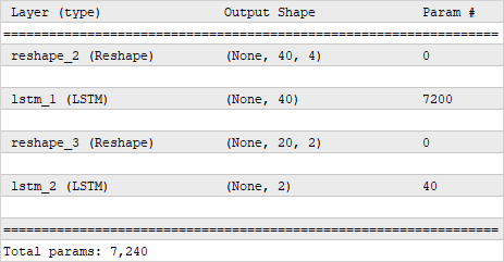
The structure of a recurrent neural network without the use of fully connected layers

We compile and train the model with the same parameters as all previous models.

model4.compile(optimizer='Adam',
loss='mean_squared_error',
metrics=['accuracy'])

history4 = model4.fit(train_data, train_target,
                      epochs=500, batch_size=1000,
                      callbacks=[callback],
                      verbose=2,
                      validation_split=0.01,
                      shuffle=False)

In the second recurrent model, to create the input tensor for the second LSTM layer, we reshaped the tensor of results from the previous layer. The Keras library gives us another option. In the first LSTM layer, we can specify the parameter return_sequences=True, which switches the recurrent layer to a mode that outputs results at each iteration. As a result of this action, at the output of the recurrent layer, we immediately obtain a three-dimensional tensor of the format [batch, timesteps, feature]. This will allow us to avoid reformatting the data before the second recurrent layer.

# LSTM model block without fully connected layers
model5 = keras.Sequential([keras.Input(shape=inputs),
# Reformat the tensor to 3-dimensional.
# Specify 2 dimensions, because. The 3rd dimension is determined by the size of the packet
                           keras.layers.Reshape((-1,4)),
# 2 Serial LSTM Units
#1st contains 40 items and returns the result at each step
                           keras.layers.LSTM(40,
               kernel_regularizer=keras.regularizers.l1_l2(l1=1e-7, l2=1e-5),
                           return_sequences=True),
# 2nd produces the result instead of a fully connected layer
                           keras.layers.LSTM(targerts)
                         ])

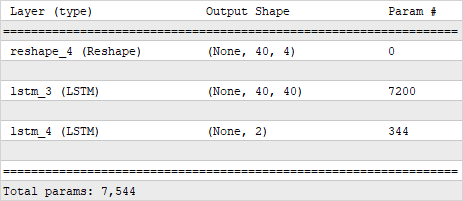
The structure of a recurrent neural network without the use of fully connected layers

As you can see, with this model construction, the dimensionality of the tensor at the output of the first recurrent layer has changed. As a result, the number of parameters in the second recurrent layer has slightly increased. This resulted in a total increase in parameters throughout the model, reaching 7,544 parameters. Nevertheless, this is still fewer parameters than the total number of parameters in the first recurrent model that used a perceptron for decision-making.

Let's supplement the plotting block with new models.

# Rendering model training results
plt.figure()
plt.plot(history1.history['loss'], label='Perceptron train')
plt.plot(history1.history['val_loss'], label='Perceptron validation')
plt.plot(history3.history['loss'], label='Conv2D train')
plt.plot(history3.history['val_loss'], label='Conv2D validation')
plt.plot(history2.history['loss'], label='LSTM train')
plt.plot(history2.history['val_loss'], label='LSTM validation')
plt.plot(history4.history['loss'], label='LSTM only train')
plt.plot(history4.history['val_loss'], label='LSTM only validation')
plt.plot(history5.history['loss'], label='LSTM sequences train')
plt.plot(history5.history['val_loss'], label='LSTM sequences validation')
plt.ylabel('$MSE$ $loss$')
plt.xlabel('$Epochs$')
plt.title('Model training dynamics')
plt.legend(loc='upper right', ncol=2)

plt.figure()
plt.plot(history1.history['accuracy'], label='Perceptron train')
plt.plot(history1.history['val_accuracy'], label='Perceptron validation')
plt.plot(history3.history['accuracy'], label='Conv2D train')
plt.plot(history3.history['val_accuracy'], label='Conv2D validation')
plt.plot(history2.history['accuracy'], label='LSTM train')
plt.plot(history2.history['val_accuracy'], label='LSTM validation')
plt.plot(history4.history['accuracy'], label='LSTM only train')
plt.plot(history4.history['val_accuracy'], label='LSTM only validation')
plt.plot(history5.history['accuracy'], label='LSTM sequences train')
plt.plot(history5.history['val_accuracy'], label='LSTM sequences validation')
plt.ylabel('$Accuracy$')
plt.xlabel('$Epochs$')
plt.title('Model training dynamics')
plt.legend(loc='lower right', ncol=2)

Additionally, let's add the new models to the testing block to evaluate their performance on the test dataset and display the results.

# Check the results of models on a test sample
test_loss1, test_acc1 = model1.evaluate(test_data, test_target, verbose=2)
test_loss2, test_acc2 = model2.evaluate(test_data, test_target, verbose=2)
test_loss3, test_acc3 = model3.evaluate(test_data, test_target, verbose=2)
test_loss4, test_acc4 = model4.evaluate(test_data, test_target, verbose=2)
test_loss5, test_acc5 = model5.evaluate(test_data, test_target, verbose=2)

print('LSTM model')
print('Test accuracy:', test_acc2)
print('Test loss:', test_loss2)

print('LSTM only model')
print('Test accuracy:', test_acc4)
print('Test loss:', test_loss4)

print('LSTM sequences model')
print('Test accuracy:', test_acc5)
print('Test loss:', test_loss5)

In this section, we have prepared a Python script that creates a total of 5 neural network models:

Fully connected perceptron
Convolutional model
3 models of recurrent neural networks

Upon executing the script, we will conduct a brief training of all five models using a single dataset and then compare the performance of the trained models on a shared set of test data. This will give us the opportunity to compare the performance of various architectural solutions on real data. The test results will be provided in the next chapter.

Implementing recurrent models in Python

Comparative testing of recurrent models