Comparative testing of recurrent models
Finally we have reached the testing phase of recurrent models. Previously, we have already tested various fully connected perceptron models and several convolutional models. You may notice that in both sections devoted to testing models, there is a certain sequence of actions, that is, a specific testing algorithm. In this section, we will follow this sequence.
As with the testing of previous models, we will start by checking the correctness of the gradient distribution through our recurrent layer built in MQL5. To do this, we will create the check_gradient_lstm.mq5 script based on previously created similar scripts for testing the correctness of the performance of previous models. Basically, we will make a copy of the script check_gradient_conv.mq5 from the convolutional model testing section and make changes to match the new model.
The change we will make in the script is the block defining the model structure for testing. We will remove the convolutional and pooling layers from the model. Instead, our model will feature one recurrent layer.
//--- recurrent layer
|
The rest of the neural network building block remains unchanged.
When testing other architectural solutions of neural layer configurations, the modifications to the script provided above in terms of defining the neural network structure would be sufficient for conducting the test. But the LSTM recurrent block has its own peculiarities. First, it lacks a weight matrix in the conventional sense. Instead, its functionality is assigned to the weight matrices of the inner layers. It will be a little more difficult to organize access to them, but I do not see the point in doing this. For inner layers, we utilize a previously validated fully connected layer class, the proper functioning of which we are confident in. Therefore, there is no need for us to retest the functioning of the already validated algorithm for gradient error distribution to the weight matrix. At the same time, we have a question about the correctness of the new functionality for the distribution of the error gradient inside the LSTM block. I believe that to answer this question, it is sufficient to verify the propagation of the error gradient back to the level of the original data (input of the neural network). Hence, we are removing the gradient error correctness checking block at the weight matrix level from the script.
The second feature of the recurrent layer is the use of its results as input for the new iteration, which is the desired feature. We wanted the neural network to consider not only the current state of the external environment but also its previous states, which we pass as hidden states to the new iteration. While this approach yields a positive impact on the neural network performance, it does distort the data for testing the correctness of gradient error distribution. The reason is that our entire algorithm for testing the correctness of gradient error distribution is built on the principle of changing only one tested parameter while keeping other values of the external environment constant. However, with a recurrent layer, even when all parameters of the input data remain constant, we can obtain a different result due to changes in the hidden state. To exclude this influence, we temporarily need to add a memory buffer and hidden state clearing within the forward pass method of our recurrent LSTM block class CNeuronLSTM::FeedForward.
bool CNeuronLSTM::FeedForward(CNeuronBase *prevLayer)
|
Don't forget to remove or comment out these lines after running the gradient propagation test.
After making all the necessary adjustments, we will compile and initiate the test execution using the OpenCL multi-threaded computation technology and without it. The results obtained fully satisfy our requirements and we can continue testing the models further.

Correctness Test of Error Gradient Distribution via LSTM Block
We have obtained confirmations of the correctness of the algorithm we built for propagating gradient error through the recurrent LSTM block. Now we can proceed to the next stage of our tests. But once again, before starting work on conducting tests, we need to remove the above code for resetting memory buffers and hidden state from the code of the direct CNeuronLSTM::FeedForward method.
Script for testing recurrent models
Let's create the script lstm_test.mq5 to test train the recurrent model. This script is created following the template of scripts used for similar testing of previous models.
At the beginning of the script, we declare external parameters to control the process of creating and training the neural network model. Almost all external parameters migrated from the script for testing convolutional models without changes.
//+------------------------------------------------------------------+
|
In the CreateLayersDesc model architecture description function, we insert one LSTM block between the source data layer and the block of hidden layers. The size of the result buffer for this recurrent block will be equal to the number of analyzed neural layers. The depth of the analyzed history will be set to five iterations. The architecture of the LSTM block defines the activation functions for all its components, and the block itself does not have a top-level activation function. Consequently, in the description of the block architecture, we will specify the absence of an activation function. We will use Adam as a method of parameter optimization.
//--- recurrent layer
|
The process of creating a recurrent neural network model can be considered completed, since the rest of the function code has remained unchanged.
At this stage of script execution, we already have a constructed recurrent neural network model and the training dataset loaded into memory. Now we can say that we are ready to train the model. And here we will have a slight departure from the previously used template. The reason is that for training the fully connected perceptron and the convolutional neural network, we used random patterns from the overall training dataset. At the same time, we've mentioned multiple times that recurrent neural networks require strict adherence to the chronological sequence of inputted raw data. Therefore, we have to make small changes to the training function of the NetworkFit model.
We need a strict sequence of patterns when training a model. Therefore, we remove the generation of a random pattern for each iteration. Instead, we will randomly determine the start of the next data batch from the training dataset.
bool NetworkFit(CNet &net, const CArrayObj &data, const CArrayObj &target,
|
But there is a nuance here as well. During the feed-forward pass, the recurrent block takes into account the results of previous iterations to the depth of the analyzed history. For the sake of data comparability, we should fill the buffer with sequential data before training the model. Therefore, we extend the loop of each batch before updating the parameters by the number of iterations required to fill the buffer with the depth of the analyzed history. In this case, we will not call the backpropagation method until the buffer is full.
for(int i = 0; (i < (BatchSize + 10) && (k + i) < patterns); i++)
|
The rest of the script code remained unchanged.
I hope that everything is clear with the algorithm and the principle of constructing the script, and we can proceed to the analysis of the results.
Testing the LSTM for the first time
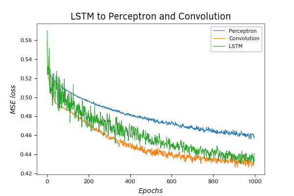
First, I created a model similar to the convolutional models I tested: one recurrent layer, three hidden fully connected layers, and one fully connected layer to display the results.
Based on the test results, it can be observed that using a recurrent layer alongside a convolutional layer for data preprocessing significantly improves the performance quality of the fully connected perceptron.
Let me remind you that in the perceptron model we used three hidden fully connected layers and one fully connected results layer. In the convolutional network model, we employed one convolutional layer, one pooling layer, three hidden fully connected layers, and one fully connected layer for output results. In the recurrent neural network model, we utilized one recurrent LSTM block, three hidden fully connected layers, and one fully connected layer for output results.
Essentially, in the convolutional and recurrent models, we introduced a convolutional or recurrent block before the previously tested perceptron for data preprocessing. The type of block used depends on the model.
As a result, we see an improvement in neural performance due to an additional layer of preliminary data processing.
Testing a Recurrent Neural Network Model
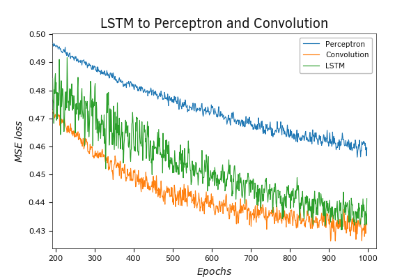
Comparing the convolutional and recurrent models, it can be observed that the error graph of the recurrent model exhibits larger noisy fluctuations. This may be due to the peculiarities of model training. To train the convolutional model, we used patterns randomly selected from the entire training set. This approach provides the most representative sample for each gradient error accumulation batch before updating the weights. At the same time, for training the recurrent model, we took patterns in chronological order. Consequently, the updating of weights and the recording of the model average error were done at different time intervals. This could not have gone unnoticed in the results, as each local time interval is subject to its own local trends.
Testing a Recurrent Neural Network Model
Despite the large graph noise, the overall trend of the recursive model has a large tendency to reduce the error. True, throughout the training process, the model error value is slightly better for the convolutional model. But after 700 iterations of updating the weight matrix of the model, there is a noticeable trend towards a slowdown in the error reduction rate. This may indicate an approach to a minimum. At the same time, the recurrent model does not have such a trend. The recurrent model has a large number of parameters, and it takes more time to train. Potentially, it can improve the results in further training.
Second test of the LSTM mode
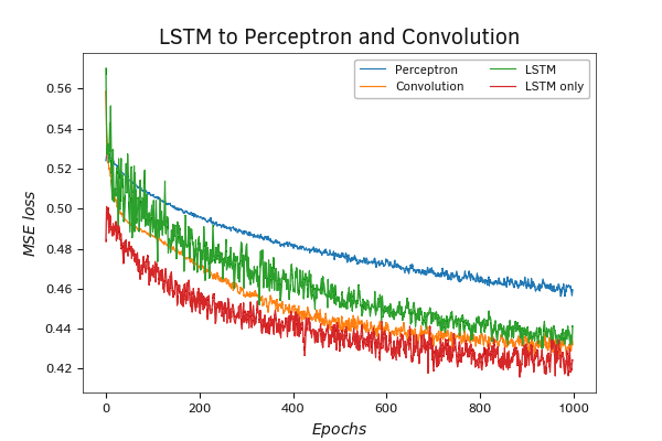
In the previous testing of the recurrent model, we used an LSTM layer to preprocess the initial data before a block of fully connected neural layers. But in practice, there is the possibility of using recurrent layers without additional preprocessing. To assess the impact of the fully connected layer block on the performance quality of the recurrent neural network, we conducted a second experiment using the same script. However, now we have specified 0 in the number of hidden layers parameter. Thus, we aim to compare the performance of two recurrent models and evaluate the necessity of using a block of fully connected neural layers for further data processing after the recurrent layer.
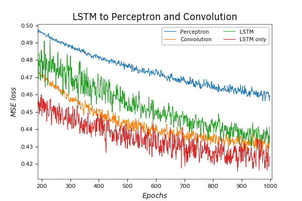
The test results show a very interesting trend. At the beginning of training, the recurrent model without hidden fully connected layers demonstrates a sharper drop in model error, surpassing all other models depicted on the graph. When you zoom in on the graph, you can see a clear advantage of the model without a block of hidden fully connected layers.
Testing a Recurrent Neural Network Model
Testing a Recurrent Neural Network Model
The results of the tests show the advantage of the operation of recurrent networks over the previously considered models. In this case, the use of recurrent layers yields results even without the additional processing of results by fully connected layers.
Here it must be noted that the evaluation of models was carried out only to solve a specific problem of working with time series. When solving other problems, it is possible to obtain absolutely opposite results. Therefore, when tackling your tasks, it is recommended to experiment with various architectural solutions for neural networks.
Results of testing recurrent models in Python
Earlier, we considered the implementation of a script with the construction of three recurrent models in Python. Now I propose to consider the results of test training of the constructed models.
The obtained testing results confirm the conclusions we made earlier based on the testing of models created using MQL5 tools. All three recurrent models are significantly superior to other models in terms of the quality of the neural network. In the graph depicting the change in error during the neural network training process, we can observe that the recurrent models already demonstrate lower error after 50 epochs of training compared to the fully connected perceptron and the convolutional model. With further training, superiority only grows. At the same time, one can also notice an increase in the error on the validation set, which indicates the tendency of the model to overfit.
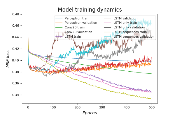
Test training results for Python models
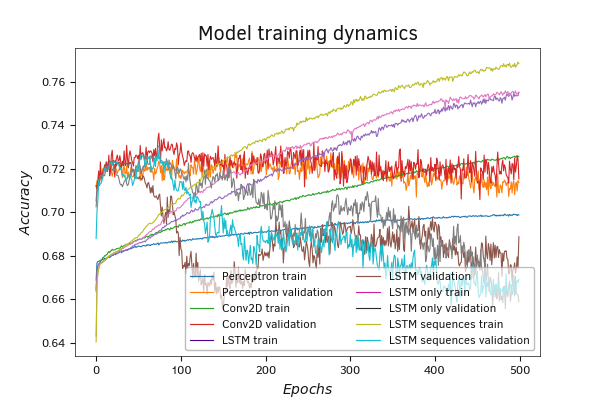
Test training results for Python models
Comparing the recurrent models with each other, you can see that the recurrent model in which the first recurrent layer returns values on each cycle is more prone to overfitting. It shows the smallest error of all models on the training set and the maximum error on the validation set. At the same time, the intersection of error curves on the testing and validation datasets for the mentioned model occurs around 130 epochs with an error value of approximately 0.385. The intersection of the graphs of the other two models is observed with an error level of about 0.395.
The graph of the dynamics of learning by the Accuracy metric fully confirms our conclusions made on the error graph.
On the test set, all trained models showed fairly close results. The deviation in both the root-mean-square error and the accuracy metric is minimal.
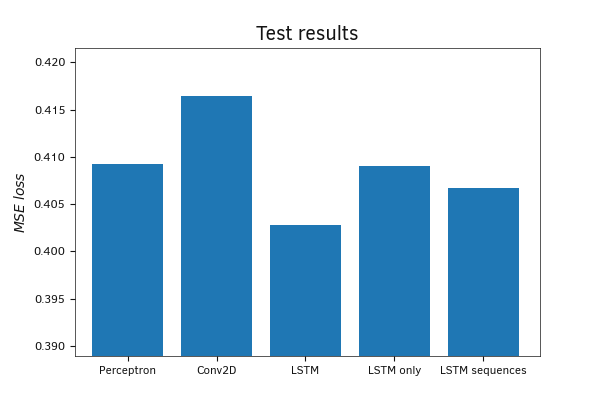
Testing Trained Python Models on a Test Set
While the picture is quite mixed in terms of MSE values, a clear superiority of the recurrent models is evident on the Accuracy metric graph.
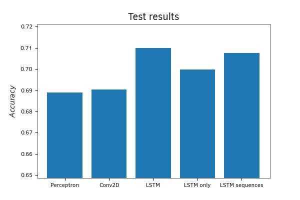
Testing Trained Python Models on a Test Set
Based on the conducted tests, it can be concluded that when dealing with time series tasks, recurrent networks are capable of producing better results than the previously examined architectural solutions. At the same time, to solve such problems, we can consider various architectural solutions. Among these solutions, there could be neural networks consisting solely of recurrent layers, or mixed models that combine layers of different types.
Despite the fact that our Python language model test resulted in the victory of a recurrent model containing only recurrent neural layers, I recommend that when tackling your practical tasks, you always experiment with different models. Often, the best results come from the most unconventional architectural solutions.