Market phenomena - page 33
You are missing trading opportunities:
- Free trading apps
- Over 8,000 signals for copying
- Economic news for exploring financial markets
Registration
Log in
You agree to website policy and terms of use
If you do not have an account, please register
Not that it's wrong. Right, as right as the expression 'buy cheap, sell dear'. It's not just correctness that matters, it's also formalisability. There is no point in constructing clever philosophical near-market constructs if they (constructs) are like the milk of a goat.
Do you think that the time lapse after accepting a loss is difficult to formalise? Or what is different?
Thanks. I'll be thinking about SOM at my leisure.
The article at the link provides an overview of time series segmentation methods. They all do about the same thing. Not that SOM is the best method for forex, but it's not the worst either, that's a fact ))
http://citeseerx.ist.psu.edu/viewdoc/download?doi=10.1.1.115.6594&rep=rep1&type=pdf
My colleagues, unfortunately, do not allow me to give more time to trading, but I found some time and decided to ask (for my own interest, so I won't forget it :o, so I will come back later, when I have more free time)
The essence of the phenomenon.
Let me remind you the essence of this phenomenon. It was discovered during analysis of "long tails" influence on future price deviations. If we classify long tails and look at the time series without them, we can observe some curious phenomena, unique for almost each symbol. The essence of the phenomenon is a very specific classification, based in some way on a "neural" approach. In fact, this classification "breaks down" the raw data, i.e. the quoting process itself into two sub-processes, which are conventionally called "alpha" and "betta". Generally speaking, the initial process can be broken down into more subprocesses.
System with random structure
This phenomenon applies very well to systems with random structure. The model itself will look very simple. Let us have a look at an example. The initial EURUSD series M15(we need a long sample, and as small as possible frame), from some "now":
Step 1: Classification
Classification is performed and two processes "alpha" and "beta" are obtained. Parameters of the control process are defined (the process, which deals with final "assembling" of the quote)
Step 2 Identification
For each sub-process a model based on the Volterry network is defined:
Oh what a pain to identify them.
Step 3 Sub-process prediction
A forecast is made for 100 counts for each process (for 15 minutes, i.e. just over a day).
Step 4: Simulation modeling
A simulation model is built, which will generate the x.o. number of future implementations. The scheme of the system is simple:
Three randomisations: an error for each model and process transition conditions. Here are the realisations themselves (from zero):
Step 5: The trading solution.
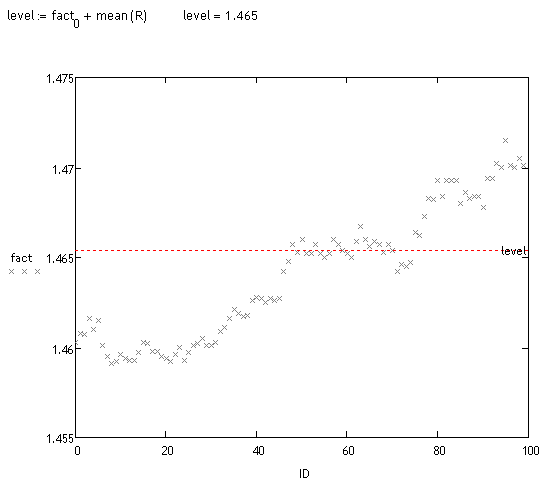
A bias analysis of these realizations is performed. This can be done in different ways. Visually, you can see that a large mass of trajectories are shifted. Let's look at the fact:
<>
Preliminary testing
Took about 70 "measurements" at random (takes a long time to count). About 70% of deviation detected by the system is correct, so it hasn't said anything yet, but I hope to get back to this track in a couple of months, although I have not finished working on the main project yet :o(.
to sayfuji
Может не совсем корректно: по какому принципу производится классификация и, собственно, разложение на какие процессы предполагается?
No, everything is correct. It was one of the subjects of discussion on several dozen pages of this thread. All that I considered necessary - I wrote. Unfortunately, I have no time to develop the topic further. Besides, this phenomenon in particular, though interesting, is not very promising. The phenomenon of "long tails" appears on long horizons, i.e. where there are large deviations of trajectories, but for this purpose it is necessary to forecast far away the processes alpha and betta (and other processes). And this is impossible. There is no such technology...
:о(
to All
Colleagues, it turns out that there are posts I haven't answered. Forgive me, there's no point in trying to move now.
Prohwessor Fransfort, please answer which program you use for your research.
And also...if anyone has a manual in Russian or a russifier for the program http://originlab.com/ (OriginPro 8.5.1)
An interesting result.
Could this phenomenon be due to the fact that the historical data are Bid prices? (Lambda in the experiment is comparable to the spread).
Don't you think it makes more sense to test the quality of the resulting "trend" process using linear regression with piecewise constant coefficients when viewed as functions of time?
You can add up the filtered increments and you get two processes: