Discussion of article "Third Generation Neural Networks: Deep Networks" - page 2

 
vlad1949:

It's not a question for me. Is that all you have to say about the article?

What about the article? It's a typical rewrite. It's the same thing in other sources, just in slightly different words. Even the pictures are the same. I didn't see anything new, i.e. authorial.

I wanted to try out the examples, but it's a bummer. The section is for MQL5, but the examples are for MQL4.


vlad1949

Dear Vlad!

Looked through the archives, you have rather old R documentation. It would be good to change to the attached copies.

Files:
Doc_R.zip  2181 kb
 

vlad1949

Dear Vlad!

Why did you fail to run in the tester?

I have everything works without problems. But the scheme is without an indicator: the Expert Advisor communicates directly with R.


Jeffrey Hinton, inventor of deep networks: "Deep networks are only applicable to data where the signal-to-noise ratio is large. Financial series are so noisy that deep networks are not applicable. We've tried it and no luck."

Listen to his lectures on YouTube.

 
gpwr:

Jeffrey Hinton, inventor of deep networks: "Deep networks are only applicable to data where the signal-to-noise ratio is large. Financial series are so noisy that deep networks are not applicable. We've tried it and no luck."

Listen to his lectures on youtube.

Considering your post in the parallel thread.

Noise is understood differently in classification tasks than in radio engineering. A predictor is considered noisy if it is weakly related (has weak predictive power) for the target variable. A completely different meaning. One should look for predictors that have predictive power for different classes of the target variable.

 
I have a similar understanding of noise. Financial series depend on a large number of predictors, most of which are unknown to us and which introduce this "noise" into the series. Using only publicly available predictors, we are unable to predict the target variable no matter what networks or methods we use.
 
gpwr:
I have a similar understanding of noise. Financial series depend on a large number of predictors, most of which are unknown to us and which introduce this "noise" into the series. Using only the publicly available predictors, we are unable to predict the target variable no matter what networks or methods we use.
See my thread.
 
faa1947:

vlad1949

Dear Vlad!

Why did you fail to run in the tester?

I have everything works without problems. True the scheme without an indicator: the advisor directly communicates with R.

llllllllllllllllllllllllllllllllllllllllllllllllllllllllllllllllllllllllllllllllllllllllllllllllllllllllllllllllllllllllllllllllllllll

Good afternoon SanSanych.

So the main idea is to make multicurrency with several indicators.

Otherwise, of course, you can pack everything into an Expert Advisor.

But if training, testing and optimisation will be implemented on the fly, without interrupting trading, then the variant with one Expert Advisor will be a bit more difficult to implement.

Good luck

PS. What is the result of testing?


Greetings SanSanych.

Here are some examples of determining the optimal number of clusters that I found on some English-speaking forum. I was not able to use all of them with my data. Very interesting 11 package "clusterSim".

--------------------------------------------------------------------------------------

#
n = 100
g = 6 
set.seed(g)
d <- data.frame(x = unlist(lapply(1:g, function(i) rnorm(n/g, runif(1)*i^2))), 
                y = unlist(lapply(1:g, function(i) rnorm(n/g, runif(1)*i^2))))
plot(d)
--------------------------------------
#1 
library(fpc)
pamk.best <- pamk(d)
cat("number of clusters estimated by optimum average silhouette width:", strpamk.best$nc, "\n")
plot(pam(d, pamk.best$nc))

#2 we could also do:
library(fpc)
asw <- numeric(20)
for (k in 2:20)
  asw[[k]] <- pam(d, k) $ silinfo $ avg.width
k.best <- which.max(asw)
cat("silhouette-optimal number of clusters:", k.best, "\n")
---------------------------------------------------
#3. Calinsky criterion: Another approach to diagnosing how many clusters suit the data. In this case 
# we try 1 to 10 groups.
require(vegan)
fit <- cascadeKM(scale(d, center = TRUE,  scale = TRUE), 1, 10, iter = 1000)
plot(fit, sortg = TRUE, grpmts.plot = TRUE)
calinski.best <- as.numeric(which.max(fit$results[2,]))
cat("Calinski criterion optimal number of clusters:", calinski.best, "\n")
# 5 clusters!
-------------------
4. Determine the optimal model and number of clusters according to the Bayesian Information 
Criterion for expectation-maximization, initialized by hierarchical clustering for parameterized 
Gaussian mixture models
library(mclust)
# Run the function to see how many clusters
# it finds to be optimal, set it to search for
# at least 1 model and up 20.
d_clust <- Mclust(as.matrix(d), G=1:20)
m.best <- dim(d_clust$z)[2]
cat("model-based optimal number of clusters:", m.best, "\n")
# 4 clusters
plot(d_clust)
----------------------------------------------------------------
5. Affinity propagation (AP) clustering, see http://dx.doi.org/10.1126/science.1136800 
library(apcluster)
d.apclus <- apcluster(negDistMat(r=2), d)
cat("affinity propogation optimal number of clusters:", length(d.apclus@clusters), "\n")
# 4
heatmap(d.apclus)
plot(d.apclus, d)
---------------------------------------------------------------------
6. Gap Statistic for Estimating the Number of Clusters. 
See also some code for a nice graphical 
output . Trying 2-10 clusters here:
library(cluster)
clusGap(d, kmeans, 10, B = 100, verbose = interactive())
-----------------------------------------------------------------------
7. You may also find it useful to explore your data with clustergrams to visualize cluster 
assignment, see http://www.r-statistics.com/2010/06/clustergram-visualization-and-diagnostics-for-cluster-analysis-r-code/&nbsp; 
for more details.
-------------------------------------------------------------------
#8. The NbClust package  provides 30 indices to determine the number of clusters in a dataset.
library(NbClust)
nb <- NbClust(d, diss = NULL, distance = "euclidean", 
        min.nc=2, max.nc=15, method = "kmeans", 
        index = "alllong", alphaBeale = 0.1)
hist(nb$Best.nc[1,], breaks = max(na.omit(nb$Best.nc[1,])))
# Looks like 3 is the most frequently determined number of clusters
# and curiously, four clusters is not in the output at all!
-----------------------------------------
Here are a few examples:
d_dist <- dist(as.matrix(d))   # find distance matrix 
plot(hclust(d_dist))           # apply hirarchical clustering and plot
----------------------------------------------------
#9 Bayesian clustering method, good for high-dimension data, more details:
# http://vahid.probstat.ca/paper/2012-bclust.pdf
install.packages("bclust")
library(bclust)
x <- as.matrix(d)
d.bclus <- bclust(x, transformed.par = c(0, -50, log(16), 0, 0, 0))
viplot(imp(d.bclus)$var); 
plot(d.bclus); 
ditplot(d.bclus)
dptplot(d.bclus, scale = 20, horizbar.plot = TRUE,varimp = imp(d.bclus)$var, horizbar.distance = 0, dendrogram.lwd = 2)
-------------------------------------------------------------------------
#10 Also for high-dimension data is the pvclust library which calculates 
#p-values for hierarchical clustering via multiscale bootstrap resampling. Here's #the example from the documentation (wont work on such low dimensional data as in #my example):
library(pvclust)
library(MASS)
data(Boston)
boston.pv <- pvclust(Boston)
plot(boston.pv)
------------------------------------
###Automatically cut the dendrogram
require(dynamicTreeCut)
ct_issues <- cutreeHybrid(hc_issues, inverse_cc_combined, minClusterSize=5)
-----
FANNY <- fanny(as.dist(inverse_cc_combined),, k = 3, maxit = 2000) 
FANNY$membership MDS <- smacofSym(distMat)$conf 
plot(MDS, type = "n") text(MDS, label = rownames(MDS), col = rgb((FANNY$membership)^(1/1)))
-----
m7 <- stepFlexmix
----------------------
#11 "clusterSim" -Department of Econometrics and Computer Science, University of #Economics, Wroclaw, Poland
http://keii.ue.wroc.pl/clusterSim
See file ../doc/clusterSim_details.pdf for further details
data.Normalization Types of variable (column) and object (row) normalization formulas
Description
Types of variable (column) and object (row) normalization formulas
Usage
data.Normalization (x,type="n0",normalization="column")
Arguments
x vector, matrix or dataset
type type of normalization: n0 - without normalization
n1 - standardization ((x-mean)/sd)
n2 - positional standardization ((x-median)/mad)
n3 - unitization ((x-mean)/range)
n3a - positional unitization ((x-median)/range)
n4 - unitization with zero minimum ((x-min)/range)
n5 - normalization in range <-1,1> ((x-mean)/max(abs(x-mean)))
n5a - positional normalization in range <-1,1> ((x-median)/max(abs(x-median)))
n6 - quotient transformation (x/sd)
n6a - positional quotient transformation (x/mad)
n7 - quotient transformation (x/range)
n8 - quotient transformation (x/max)
n9 - quotient transformation (x/mean)
n9a - positional quotient transformation (x/median)
n10 - quotient transformation (x/sum)
n11 - quotient transformation (x/sqrt(SSQ))
normalization "column" - normalization by variable, "row" - normalization by objec
See file ../doc/HINoVMod_details.pdf for further details 


In the next post calculations with my data


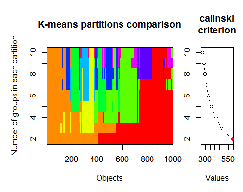
The optimal number of clusters can be determined by several packages and using more than 30 optimality criteria. According to my observations, the most used criterion is the Calinskycriterion .

Let's take the raw data from our set from the indicator dt . It contains 17 predictors, target y and candlestick body z.

In the latest versions of "magrittr" and "dplyr" packages there are many new nice features, one of them is 'pipe' - %>%. It is very convenient when you don't need to save intermediate results. Let's prepare the initial data for clustering. Take the initial matrix dt, select the last 1000 rows from it, and then select 17 columns of our variables from them. We get a clearer notation, nothing more.

> library(magrittr)
> x<-dt %>% tail( .,1000)%>% extract( ,1:17)

1.

> library(fpc)
> pamk.best <- pamk(x)
> cat("number of clusters estimated by optimum average silhouette width:", pamk.best$nc, "\n")
> number of clusters estimated by optimum average silhouette width: h: 2

2. Calinsky criterion: Another approach to diagnosing how many clusters suit the data. In this case

we try 1 to 10 groups.

> require(vegan)
> fit <- cascadeKM(scale(x, center = TRUE,  scale = TRUE), 1, 10, iter = 1000)
> plot(fit, sortg = TRUE, grpmts.plot = TRUE)

> calinski.best <- as.numeric(which.max(fit$results[2,]))
> cat("Calinski criterion optimal number of clusters:", calinski.best, "\n")
Calinski criterion optimal number of clusters: 2
3. Determine the optimal model and number of clusters according to the Bayesian InformationCriterion for expectation-maximisation, initialised by hierarchical clustering for parameterised Gaussian mixture models.

Gaussian mixture models

> library(mclust)
#  Run the function to see how many clusters
#  it finds to be optimal, set it to search for
#  at least 1 model and up 20.
> d_clust <- Mclust(as.matrix(x), G=1:20)
> m.best <- dim(d_clust$z)[2]
> cat("model-based optimal number of clusters:", m.best, "\n")
model-based optimal number of clusters: 7