Discussion of article "Deep Neural Networks (Part V). Bayesian optimization of DNN hyperparameters"
I experimented with BayesianOptimisation.
You had the largest set of 9 optimisable parameters. And you said that it takes a long time to calculate
I tried a set of 20 parameters to optimise with 10 first random sets. It took me 1.5 hours to calculate the combinations in BayesianOptimisation, without taking into account the calculation time of the NS itself (I replaced the NS with a simple mathematical formula for the experiment).
And if you want to optimise 50 or 100 parameters, it will probably take 24 hours to calculate 1 set. I think it would be faster to generate dozens of random combinations and calculate them in NS and then select the best ones by Accuracy.
The package discussion talks about this problem. A year ago the author wrote that if he finds a faster package for calculations, he will use it, but for now - as it is. There they gave a couple of links to other packages with Bayesian optimisation, but it is not clear how to apply them for a similar problem, in the examples other problems are solved.
bigGp - does not find the SN2011fe dataset for the example (apparently it was downloaded from the Internet, and the page is not available). I couldn't try the example. And according to the description - some additional matrices are required.
laGP - some confusing formula in the fitness function, and makes hundreds of its calls, and hundreds of NS calculations are unacceptable in terms of time.
kofnGA - can search only X best out of N. For example 10 out of 100. I.e. it is not optimising a set of all 100.
Genetic algorithms are not suitable either, because they also generate hundreds of calls to the fitness function (NS calculations).
In general, there is no analogue, and BayesianOptimisation itself is too long.
I experimented with BayesianOptimisation.
You had the largest set of 9 optimisable parameters. And you said it took a long time to calculate
I tried a set of 20 parameters to optimise with 10 first random sets. It took me 1.5 hours to calculate the combinations themselves in BayesianOptimisation, without taking into account the time of calculating the NS itself (I replaced the NS with a simple mathematical formula for the experiment).
And if you want to optimise 50 or 100 parameters, it will probably take 24 hours to calculate 1 set. I think it would be faster to generate dozens of random combinations and calculate them in NS, and then select the best ones by Accuracy.
The package discussion talks about this problem. A year ago, the author wrote that if he finds a faster package for calculations, he will use it, but for now - as it is. There they gave a couple of links to other packages with Bayesian optimisation, but it is not clear how to apply them for a similar problem, in the examples other problems are solved.
bigGp - does not find the SN2011fe dataset for the example (apparently it was downloaded from the Internet, and the page is not available). I couldn't try the example. And according to the description - some additional matrices are required.
laGP - some confusing formula in the fitness function, and makes hundreds of its calls, and hundreds of NS calculations are unacceptable in terms of time.
kofnGA - can search only X best out of N. For example 10 out of 100. I.e. it is not optimising a set of all 100.
Genetic algorithms are not suitable either, because they also generate hundreds of calls to the fitness function (NS calculations).
In general, there is no analogue, and BayesianOptimisation itself is too long.
There is such a problem. It is connected with the fact that the package is written in pure R. But the advantages of using it for me personally outweigh the time costs. There is a package hyperopt (Python)/ I have not had the chance to try it, and it is old.
But I think someone will still rewrite the package in C++. Of course, you can do it yourself, transfer some of the calculations to GPU, but it will take a lot of time. Only if I'm really desperate.
For now I will use what I have.
Good luck
I also experimented with examples from the GPfit package itself.
Here is an example of optimising 1 parameter that describes a curve with 2 vertices (the GPfit f-ya has more vertices, I left 2):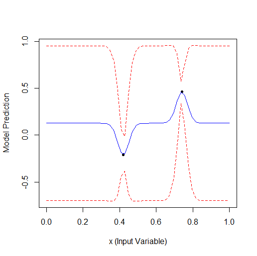
Taking 2 random points and then optimising. You can see that it finds the small vertex first and then the larger vertex. Total 9 calculations - 2 random and + 7 on optimisation.
Another example in 2D - optimising 2 parameters. The original f-y looks like this: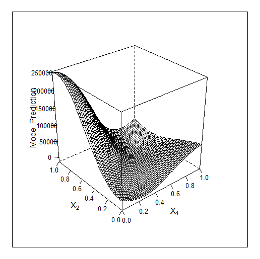
Optimisation to 19 points:
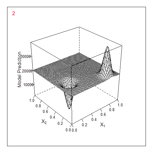
Total 2 random points + 17 found by the optimiser.
Comparing these 2 examples we can see that the number of iterations needed to find the maximum when adding 1 parameter doubles. For 1 parameter the maximum was found for 9 calculated points, for 2 parameters for 19.
I.e. if you optimise 10 parameters, you may need 9 * 2^10 = 9000 calculations.
Although at 14-points the algorithm almost found the maximum, this is about 1.5 times the number of calculations. then 9 * 1.5:10 = 518 calculations. Also a lot, for an acceptable calculation time.
The results obtained in the article for 20 - 30 points may be far from the real maximum.
I think that genetic algorithms even with these simple examples will need much more points to calculate. So there is probably no better option.
I also experimented with examples from the GPfit package itself.
Here is an example of optimising 1 parameter that describes a curve with 2 vertices (the GPfit f-ya has more vertices, I left 2):
Taking 2 random points and then optimising. You can see that it finds the small vertex first and then the larger vertex. Total 9 calculations - 2 random and + 7 on optimisation.
Another example in 2D - optimising 2 parameters. The original f-ya looks like this:
Optimise up to 19 points:
Total 2 random points + 17 found by the optimiser.
Comparing these 2 examples we can see that the number of iterations needed to find the maximum when adding 1 parameter doubles. For 1 parameter the maximum was found for 9 calculated points, for 2 parameters for 19.
I.e. if you optimise 10 parameters, you may need 9 * 2^10 = 9000 calculations.
Although at 14-points the algorithm almost found the maximum, this is about 1.5 times the number of calculations. then 9 * 1.5:10 = 518 calculations. Also a lot, for an acceptable computation time.
1. The results obtained in the article for 20 - 30 points may be far from the real maximum.
I think that genetic algorithms even with these simple examples will need to calculate many more points. So I guess there is no better option after all.
Bravo.
Clearly.
There are a number of lectures on YouTube explaining how Bayesian optimisation works. If you haven't seen it, I suggest you watch it. It's very informative.
How did you insert animation?
I try to use Bayesian methods wherever possible. The results are very good.
1. I do sequential optimisation. First - initialisation of 10 random points, Computation of 10-20 points, next - initialisation of 10 best results from previous optimisation, computation of 10-20 points. Typically after the second iteration, the results do not improve meaningfully.
Good luck
A number of lectures explaining how Bayesian optimisation works are posted on YouTube. If you have not seen it, I advise you to watch it. It is very informative.
I looked at the code and the result in the form of pictures (and showed it to you). The most important thing is Gaussian Process from GPfit. And the optimisation is the most usual - just use the optimiser from the standard R delivery and look for the maximum on the curve/shape that GPfit came up with by 2, 3, etc. points. And what it has come up with can be seen in the animated pictures above. The optimiser is just trying to get out the top 100 random points.
Maybe I will watch lectures in the future, when I have time, but for now I will just use GPfit as a black box.
How did you insert animation?
I just displayed the result step by step GPfit::plot.GP(GP, surf_check = TRUE), pasted it into Photoshop and saved it there as an animated GIF.
following - initialisation of the 10 best results from the previous optimization, calculations of 10-20 points.
According to my experiments, it is better to leave all known points for future calculations, because if the lower ones are removed, GPfit may think that there are interesting points and will want to calculate them, i.e. there will be repeated runs of NS calculation. And with these lower points, GPfit will know that there is nothing to look for in these lower regions.
Although if the results do not improve much, it means that there is an extensive plateau with small fluctuations.
How to Installation and launching ?
).

- 2016.04.26
- Vladimir Perervenko
- www.mql5.com
Forward testing the models with optimal parameters
Let us check how long the optimal parameters of DNN will produce results with acceptable quality for the tests of "future" quotes values. The test will be performed in the environment remaining after the previous optimizations and testing as follows.
Use a moving window of 1350 bars, train = 1000, test = 350 (for validation — the first 250 samples, for testing — the last 100 samples) with step 100 to go through the data after the first (4000 + 100) bars used for pretraining. Make 10 steps "forward". At each step, two models will be trained and tested:
- one — using the pretrained DNN, i.e., perform a fine-tuning on a new range at each step;
- second — additionally training the DNN.opt, obtained after optimization at the fine-tuning stage, on a new range.
#---prepare----
evalq({
  step <- 1:10
  dt <- PrepareData(Data, Open, High, Low, Close, Volume)
  DTforv <- foreach(i = step, .packages = "dplyr" ) %do% {
        SplitData(dt, 4000, 1000, 350, 10, start = i*100) %>%
        CappingData(., impute = T, fill = T, dither = F, pre.outl = pre.outl)%>%
        NormData(., preproc = preproc) -> DTn
                foreach(i = 1:4) %do% {
                DTn[[i]] %>% dplyr::select(-c(v.rstl, v.pcci))
                                } -> DTn
                list(pretrain = DTn[[1]],
                          train = DTn[[2]],
                          val =  DTn[[3]],
                          test =  DTn[[4]]) -> DTn
                list(
                        pretrain = list(
                          x = DTn$pretrain %>% dplyr::select(-c(Data, Class)) %>% as.data.frame(),
                          y = DTn$pretrain$Class %>% as.data.frame()
                        ),
                        train = list(
                          x = DTn$train %>% dplyr::select(-c(Data, Class)) %>% as.data.frame(),
                          y = DTn$train$Class %>% as.data.frame()
                        ),
                        test = list(
                          x = DTn$val %>% dplyr::select(-c(Data, Class)) %>% as.data.frame(),
                          y = DTn$val$Class %>% as.data.frame()
                        ),
                        test1 = list(
                          x = DTn$test %>% dplyr::select(-c(Data, Class)) %>% as.data.frame(),
                          y = DTn$test$Class %>% as.vector()
                        )
                  )
                }
}, env)
Perform the first part of the forward test using the pretrained DNN and optimal hyperparameters, obtained from the training variant SRBM + upperLayer + BP.
#----#---SRBM + upperLayer + BP----
evalq({
    #--BestParams--------------------------
          best.par <- OPT_Res3$Best_Par %>% unname
          # n1, n2, fact1, fact2, dr1, dr2, Lr.rbm , Lr.top, Lr.fine
          n1 = best.par[1]; n2 = best.par[2]
          fact1 = best.par[3]; fact2 = best.par[4]
          dr1 = best.par[5]; dr2 = best.par[6]
          Lr.rbm = best.par[7]
          Lr.top = best.par[8]
          Lr.fine = best.par[9]
          Ln <- c(0, 2*n1, 2*n2, 0)
  foreach(i = step, .packages = "darch" ) %do% {
          DTforv[[i]] -> X
          if(i==1) Res3$Dnn -> Dnn
          #----train/test-------
          fineTuneBP(Ln, fact1, fact2, dr1, dr2, Dnn, Lr.fine) -> Dnn.opt
      predict(Dnn.opt, newdata = X$test$x %>% tail(100) , type = "class") -> Ypred
      yTest <- X$test$y[ ,1] %>% tail(100)
      #numIncorrect <- sum(Ypred != yTest)
      #Score <- 1 - round(numIncorrect/nrow(xTest), 2)
      Evaluate(actual = yTest, predicted = Ypred)$Metrics[ ,2:5] %>%
      round(3)
  } -> Score3_dnn
 }, env)
The second stage of the forward test using Dnn.opt obtained during optimization:
evalq({
  foreach(i = step, .packages = "darch" ) %do% {
          DTforv[[i]] -> X
          if(i==1) {Res3$Dnn.opt -> Dnn}
          #----train/test-------
          fineTuneBP(Ln, fact1, fact2, dr1, dr2, Dnn, Lr.fine) -> Dnn.opt
      predict(Dnn.opt, newdata = X$test$x %>% tail(100) , type = "class") -> Ypred
      yTest <- X$test$y[ ,1] %>% tail(100)
      #numIncorrect <- sum(Ypred != yTest)
      #Score <- 1 - round(numIncorrect/nrow(xTest), 2)
      Evaluate(actual = yTest, predicted = Ypred)$Metrics[ ,2:5] %>%
      round(3)
  } -> Score3_dnnOpt
}, env)
Compare the testing results, placing them in a table:
env$Score3_dnn
env$Score3_dnnOpt
| iter | Score3_dnn | Score3_dnnOpt |
|---|---|---|
| Accuracy Precision Recall F1 | Accuracy Precision Recall F1 | |
| 1 | -1 0.76 0.737 0.667 0.7 1 0.76 0.774 0.828 0.8 | -1 0.77 0.732 0.714 0.723 1 0.77 0.797 0.810 0.803 |
| 2 | -1 0.79 0.88 0.746 0.807 1 0.79 0.70 0.854 0.769 | -1 0.78 0.836 0.78 0.807 1 0.78 0.711 0.78 0.744 |
| 3 | -1 0.69 0.807 0.697 0.748 1 0.69 0.535 0.676 0.597 | -1 0.67 0.824 0.636 0.718 1 0.67 0.510 0.735 0.602 |
| 4 | -1 0.71 0.738 0.633 0.681 1 0.71 0.690 0.784 0.734 | -1 0.68 0.681 0.653 0.667 1 0.68 0.679 0.706 0.692 |
| 5 | -1 0.56 0.595 0.481 0.532 1 0.56 0.534 0.646 0.585 | -1 0.55 0.578 0.500 0.536 1 0.55 0.527 0.604 0.563 |
| 6 | -1 0.61 0.515 0.829 0.636 1 0.61 0.794 0.458 0.581 | -1 0.66 0.564 0.756 0.646 1 0.66 0.778 0.593 0.673 |
| 7 | -1 0.67 0.55 0.595 0.571 1 0.67 0.75 0.714 0.732 | -1 0.73 0.679 0.514 0.585 1 0.73 0.750 0.857 0.800 |
| 8 | -1 0.65 0.889 0.623 0.733 1 0.65 0.370 0.739 0.493 | -1 0.68 0.869 0.688 0.768 1 0.68 0.385 0.652 0.484 |
| 9 | -1 0.55 0.818 0.562 0.667 1 0.55 0.222 0.500 0.308 | -1 0.54 0.815 0.55 0.657 1 0.54 0.217 0.50 0.303 |
| 10 | -1 0.71 0.786 0.797 0.791 1 0.71 0.533 0.516 0.525 | -1 0.71 0.786 0.797 0.791 1 0.71 0.533 0.516 0.525 |
The table shows that the first two steps produce good results. The quality is actually the same at the first two steps of both variants, and then it falls. Therefore, it can be assumed that after optimization and testing, DNN will maintain the quality of classification at the level of the test set on at least 200-250 following bars.
There are many other combinations for additional training of models on forward tests mentioned in the previous articleand numerous adjustable hyperparameters.
Hi, What's the question?
Hello Vladimir,
I don't quite understand why your NS is trained on training data and its evaluation is done on test data (if I'm not mistaken you use it as a validation one).
    Score <- Evaluate(actual = yTest, predicted = Ypred)$Metrics[ ,2:5] %>%
      round(3)
In this case, won't you get a fit to the test plot, i.e. will you choose the model that worked best on the test plot?
We should also take into account that the test plot is rather small and it is possible to fit one of the temporal regularities, which may stop working very quickly.
Maybe it is better to estimate on the training plot, or on the sum of plots, or as in Darch, (with validation data submitted) on Err = (ErrLeran * 0.37 + ErrValid * 0.63) - these coefficients are default, but they can be changed.
There are many options and it's not clear which one is best. Your arguments in favour of the test plot are interesting.
- Free trading apps
- Over 8,000 signals for copying
- Economic news for exploring financial markets
You agree to website policy and terms of use
New article Deep Neural Networks (Part V). Bayesian optimization of DNN hyperparameters has been published:
The article considers the possibility to apply Bayesian optimization to hyperparameters of deep neural networks, obtained by various training variants. The classification quality of a DNN with the optimal hyperparameters in different training variants is compared. Depth of effectiveness of the DNN optimal hyperparameters has been checked in forward tests. The possible directions for improving the classification quality have been determined.
The result is good. Let us plot a graph of training history:
plot(env$Res1$Dnn.opt, type = "class")Fig.2. History of DNN training by variant SRBM + RP
As it can be seen from the figure, the error on the validation set is less than error on the training set. This means that the model is not overfitted and has a good generalizing ability. The red vertical line indicates the results of the model that is deemed the best and returned as a result after training.
For other three training variants, only the results of calculations and history graphs without further details will be provided. Everything is calculated similarly.
Author: Vladimir Perervenko