#
n = 100
g = 6
set.seed(g)
d <- data.frame(x = unlist(lapply(1:g, function(i) rnorm(n/g, runif(1)*i^2))),
y = unlist(lapply(1:g, function(i) rnorm(n/g, runif(1)*i^2))))
plot(d)
--------------------------------------
#1
library(fpc)
pamk.best <- pamk(d)
cat("number of clusters estimated by optimum average silhouette width:", strpamk.best$nc, "\n")
plot(pam(d, pamk.best$nc))
#2 we could also do:
library(fpc)
asw <- numeric(20)
for (k in 2:20)
asw[[k]] <- pam(d, k) $ silinfo $ avg.width
k.best <- which.max(asw)
cat("silhouette-optimal number of clusters:", k.best, "\n")
---------------------------------------------------
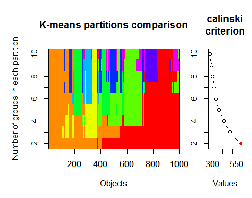
#3. Calinsky criterion: Another approach to diagnosing how many clusters suit the data. In this case
# we try 1 to 10 groups.
require(vegan)
fit <- cascadeKM(scale(d, center = TRUE, scale = TRUE), 1, 10, iter = 1000)
plot(fit, sortg = TRUE, grpmts.plot = TRUE)
calinski.best <- as.numeric(which.max(fit$results[2,]))
cat("Calinski criterion optimal number of clusters:", calinski.best, "\n")
# 5 clusters!
-------------------
4. Determine the optimal model and number of clusters according to the Bayesian Information
Criterion for expectation-maximization, initialized by hierarchical clustering for parameterized
Gaussian mixture models
library(mclust)
# Run the function to see how many clusters
# it finds to be optimal, set it to search for
# at least 1 model and up 20.
d_clust <- Mclust(as.matrix(d), G=1:20)
m.best <- dim(d_clust$z)[2]
cat("model-based optimal number of clusters:", m.best, "\n")
# 4 clusters
plot(d_clust)
----------------------------------------------------------------
5. Affinity propagation (AP) clustering, see http://dx.doi.org/10.1126/science.1136800
library(apcluster)
d.apclus <- apcluster(negDistMat(r=2), d)
cat("affinity propogation optimal number of clusters:", length(d.apclus@clusters), "\n")
# 4
heatmap(d.apclus)
plot(d.apclus, d)
---------------------------------------------------------------------
6. Gap Statistic for Estimating the Number of Clusters.
See also some code for a nice graphical
output . Trying 2-10 clusters here:
library(cluster)
clusGap(d, kmeans, 10, B = 100, verbose = interactive())
-----------------------------------------------------------------------
7. You may also find it useful to explore your data with clustergrams to visualize cluster
assignment, see http://www.r-statistics.com/2010/06/clustergram-visualization-and-diagnostics-for-cluster-analysis-r-code/
for more details.
-------------------------------------------------------------------
#8. The NbClust package provides 30 indices to determine the number of clusters in a dataset.
library(NbClust)
nb <- NbClust(d, diss = NULL, distance = "euclidean",
min.nc=2, max.nc=15, method = "kmeans",
index = "alllong", alphaBeale = 0.1)
hist(nb$Best.nc[1,], breaks = max(na.omit(nb$Best.nc[1,])))
# Looks like 3 is the most frequently determined number of clusters
# and curiously, four clusters is not in the output at all!
-----------------------------------------
Here are a few examples:
d_dist <- dist(as.matrix(d)) # find distance matrix
plot(hclust(d_dist)) # apply hirarchical clustering and plot
----------------------------------------------------
#9 Bayesian clustering method, good for high-dimension data, more details:
# http://vahid.probstat.ca/paper/2012-bclust.pdf
install.packages("bclust")
library(bclust)
x <- as.matrix(d)
d.bclus <- bclust(x, transformed.par = c(0, -50, log(16), 0, 0, 0))
viplot(imp(d.bclus)$var);
plot(d.bclus);
ditplot(d.bclus)
dptplot(d.bclus, scale = 20, horizbar.plot = TRUE,varimp = imp(d.bclus)$var, horizbar.distance = 0, dendrogram.lwd = 2)
-------------------------------------------------------------------------
#10 Also for high-dimension data is the pvclust library which calculates
#p-values for hierarchical clustering via multiscale bootstrap resampling. Here's #the example from the documentation (wont work on such low dimensional data as in #my example):
library(pvclust)
library(MASS)
data(Boston)
boston.pv <- pvclust(Boston)
plot(boston.pv)
------------------------------------
###Automatically cut the dendrogram
require(dynamicTreeCut)
ct_issues <- cutreeHybrid(hc_issues, inverse_cc_combined, minClusterSize=5)
-----
FANNY <- fanny(as.dist(inverse_cc_combined),, k = 3, maxit = 2000)
FANNY$membership MDS <- smacofSym(distMat)$conf
plot(MDS, type = "n") text(MDS, label = rownames(MDS), col = rgb((FANNY$membership)^(1/1)))
-----
m7 <- stepFlexmix
----------------------
#11 "clusterSim" -Department of Econometrics and Computer Science, University of #Economics, Wroclaw, Poland
http://keii.ue.wroc.pl/clusterSim
See file ../doc/clusterSim_details.pdf for further details
data.Normalization Types of variable (column) and object (row) normalization formulas
Description
Types of variable (column) and object (row) normalization formulas
Usage
data.Normalization (x,type="n0",normalization="column")
Arguments
x vector, matrix or dataset
type type of normalization: n0 - without normalization
n1 - standardization ((x-mean)/sd)
n2 - positional standardization ((x-median)/mad)
n3 - unitization ((x-mean)/range)
n3a - positional unitization ((x-median)/range)
n4 - unitization with zero minimum ((x-min)/range)
n5 - normalization in range <-1,1> ((x-mean)/max(abs(x-mean)))
n5a - positional normalization in range <-1,1> ((x-median)/max(abs(x-median)))
n6 - quotient transformation (x/sd)
n6a - positional quotient transformation (x/mad)
n7 - quotient transformation (x/range)
n8 - quotient transformation (x/max)
n9 - quotient transformation (x/mean)
n9a - positional quotient transformation (x/median)
n10 - quotient transformation (x/sum)
n11 - quotient transformation (x/sqrt(SSQ))
normalization "column" - normalization by variable, "row" - normalization by objec
See file ../doc/HINoVMod_details.pdf for further details
> library(fpc)
> pamk.best <- pamk(x)
> cat("number of clusters estimated by optimum average silhouette width:", pamk.best$nc, "\n")
> number of clusters estimated by optimum average silhouette width: h: 2
2.卡林斯基标准:另一种诊断数据适合多少个聚类的方法。在这种情况下
我们尝试 1 到 10 个群组。
> require(vegan)
> fit <- cascadeKM(scale(x, center = TRUE,  scale = TRUE), 1, 10, iter = 1000)
> plot(fit, sortg = TRUE, grpmts.plot = TRUE)
> calinski.best <- as.numeric(which.max(fit$results[2,]))
> cat("Calinski criterion optimal number of clusters:", calinski.best, "\n")
Calinski criterion optimal number of clusters: 2
> library(mclust)
# Run the function to see how many clusters
# it finds to be optimal, set it to search for# at least 1 model and up 20.
> d_clust <- Mclust(as.matrix(x), G=1:20)
> m.best <- dim(d_clust$z)[2]
> cat("model-based optimal number of clusters:", m.best, "\n")
model-based optimal number of clusters: 7
这对我来说不是一个问题。你对这篇文章就想说这些吗?
文章怎么了?这是典型的改写其他来源的内容都一样 只是用词略有不同连图片都一样。我看不出有什么新意,也就是作者的意思。
我想试试这些示例,但很遗憾。该部分是针对 MQL5 的,但示例却是针对 MQL4 的。
vlad1949
亲爱的弗拉德
我看了一下档案,您的 R 文档比较旧。最好改成附件中的副本。
vlad1949
亲爱的弗拉德
为什么在测试器中运行失败?
我一切正常。但该方案没有指标:EA 直接与 R 通信。
深度网络的发明者杰弗里-辛顿(Jeffrey Hinton):"深度网络只适用于信噪比较大的数据。金融序列的噪声非常大,因此深度网络并不适用。我们已经试过了,但没有成功。
在 YouTube 上收听他的演讲。
深度网络的发明者杰弗里-辛顿(Jeffrey Hinton):"深度网络只适用于信噪比较大的数据。金融序列的噪声非常大,因此深度网络并不适用。我们已经试过了,但没有成功。
请在 youtube 上收听他的讲座。
考虑到您在平行主题中的帖子。
分类任务中对噪声的理解与无线电工程中不同。如果一个预测因子与目标变量的相关性很弱(预测能力很弱),那么这个预测因子就被认为是有噪声的。这是完全不同的含义。我们应该寻找对目标变量的不同类别都有预测能力的预测因子。
我对噪声也有类似的理解。金融序列依赖于大量的预测因子,其中大部分都是我们未知的,它们会给序列带来 "噪音"。仅使用公开的预测因子,无论我们使用什么网络或方法,都无法预测目标变量。
vlad1949
亲爱的弗拉德
为什么在测试器中运行失败?
我一切正常。没有指示器的方案是正确的:顾问直接与 R 通信。
llllllllllllllllllllllllllllllllllllllllllllllllllllllllllllllllllll
下午好,SanSanych。
因此,我们的主要想法是用多个指标来制作多币种。
当然,您也可以将一切都打包到 Expert Advisor 中。
但是,如果要在不中断交易的情况下随时进行培训、测试和优化,那么使用一个智能交易系统的变体就比较难以实现。
祝您好运
PS.测试结果如何?
你好,SanSanych。
下面是我在一些英语论坛上找到的一些确定最佳聚类数的示例。我无法将它们全部用于我的数据。非常有趣的 11 软件包"clusterSim"。
--------------------------------------------------------------------------------------
下一篇文章将用我的数据进行计算
最佳聚类数可以通过多个软件包并使用 30 多个优化标准来确定。根据我的观察,使用最多的标准 是卡林斯基标准 。
让我们从指标 dt 中获取原始数据 。它包含 17 个预测因子、目标 y 和蜡烛图主体 z。
在最新版本的 "magrittr " 和 "dplyr " 软件包中 ,有许多不错的新功能, 其中之一就是 "管道" - %>%。 当你不需要保存中间结果时,它非常方便。让我们为聚类准备初始数据。取初始矩阵 dt,从中选取最后 1000 行,然后从中选取 17 列变量。我们得到了一个更清晰的符号,仅此而已。
1.
2.卡林斯基标准:另一种诊断数据适合多少个聚类的方法。在这种情况下
我们尝试 1 到 10 个群组。
3.根据贝叶斯信息准则(Bayesian InformationCriterion)的期望最大化(expectation-maximisation)来确定最佳模型和聚类数量,并通过参数化高斯混合物模型的分层聚类(hierarchical clustering)进行初始化。高斯混合模型