- Description of the architecture
- Building a GPT model in MQL5
- Organizing parallel computing in the GPT model
- Comparative testing of implementations
Comparative testing of implementations
We have completed the CNeuronGPT neural layer class using the attention mechanisms. In this class, we attempted to recreate the GPT (Generative Pre-trained Transformer) model proposed by the OpenAI team in 2018. This model was developed for language tasks but later showed quite good results for other tasks as well. The third generation of this model (GPT-3) is the most advanced language model at the time of writing this book.
The distinguishing feature of this model from other variations of the Transformer model is its autoregressive algorithm. In this case, the model is not fed with the entire volume of data describing the current state but only the changes in the state. In language problem solving examples, we can input into the model not the whole text at once, but one word at a time. Furthermore, the output generated by the model represents a continuation of the sentence. We input this word again into the model without repeating the previous phrase. The model maps it to the stored previous states and generates a new word. In practice, such an autoregressive model allows the generating of coherent texts. By avoiding the reprocessing of previous states, the model's computational workload is significantly reduced without sacrificing its performance quality.
We will not set the task of generating a new chart candlestick. For a comparative analysis of the model performance with previously discussed architectural solutions, we will keep the same task and the previously used training dataset. However, we will make the task more challenging for this model. Instead of providing the entire pattern as before, we will only input a small part of it consisting of the last five candles. To do this, let's modify our test script a bit.
We will write the script for this test to the file gpt_test.mq5. As a template, we take one of the previous attention model testing scripts: attention_test.mq5. At the beginning of the script, we define a constant for specifying the size of the pattern in the training dataset file and external parameters for configuring the script.
#define GPT_InputBars 5
|
As you can see, all the external parameters of the script have been inherited from the test script of the previous model. The constant for the size of the pattern in the training dataset is necessary for organizing the correct loading of data because, in this implementation, the size of the data passed to the model will be significantly different from the size of the pattern in the training dataset. I didn't make this constant an external parameter because we are using a single training dataset, so there's no need to change this parameter during testing. At the same time, the introduction of an additional external parameter can potentially add confusion for the user.
After declaring the external parameters of the test script we are creating, we include our library for creating neural network models.
//+------------------------------------------------------------------+
|
Here we finish creating global variables and can proceed with the script.
In the body of the script, we need to make changes to two functions. The first changes will be made to the CreateLayersDesc function that describes the architecture of the model. As mentioned above, we will only feed information about the last five candlesticks to the model input. So, we reduce the size of the raw data layer to 20 neurons. But we will make the script architecture flexible and specify the size of the source data layer as the product of the external parameter of the number of neurons per description of one candlestick in NeuronsToBar and the constant of the number of candlesticks to load in GPT_InputBars.
bool CreateLayersDesc(CArrayObj &layers)
|
Note that in case of an error occurring while adding an object to the dynamic array, we output a message to the log for the user and make sure to delete the objects we created before the script finishes. It should become a good practice for you to always clean up memory before the program terminates, whether it's normal termination or due to an error.
After adding a neural layer to the dynamic array of descriptions, we proceed to the next neural layer. We create a new instance of an object to describe the neural layer. We cannot use the previously created instance because the variable only holds a pointer to the object. This same pointer was passed to the dynamic array of pointers to objects describing neural layers. Therefore, when making changes to the object through the pointer in the local variable, all new data will be reflected when accessing the object through the pointer in the dynamic array. Thus, by using one pointer, we will only have copies of the same pointer in the dynamic array, and the program will create a model consisting of identical neural layers instead of the desired architecture.
//--- GPT block
|
As the second layer, we will create a GPT block. The model will know about this from the defNeuronGPT constant in the type field of the created neural layer.
In the count field, we will specify the stack size to store the pattern information. Its value will determine the size of the buffers for the Key and Value tensors, and will also affect the size of the vector of dependency coefficients Score.
We will set the size of the input window equal to the number of elements in the previous layer, which we have saved in a local variable.
The size of the description vector of one element in the Key tensor will be equal to the number of description elements of one candlestick. This is the value we used when performing previous tests with attention models. This approach will help us to put more emphasis on the impact of the solution architecture itself, rather than the parameters used.
We also transfer the rest of the parameters unchanged from the scripts of previous tests with attention models. Among them are the number of attention heads used and the parameter optimization function. I'll remind you that the activation functions for all internal neural layers are defined by the Transformer architecture, so there's no need for an additional activation function for the neural layer here.
descr.type = defNeuronGPT;
|
Besides, when testing the Multi-Head Self-Attention architecture, we created four identical neural layers. Now, to create such an architecture, we only need to create one description of a neural layer and specify the number of identical neural layers in the layers parameter.
We add the created description of the neural layer to our collection of descriptions of the architecture of the created model.
if(!layers.Add(descr))
|
Next comes a block of hidden fully connected neural layers, transferred in an unchanged form from the scripts of the previous tests, as well as the results layer. At the output of our model, there will be a results layer represented by a fully connected neural layer with two elements and a linear activation function.
The next block we will modify is the LoadTrainingData function for loading the training sample.
First, we create two dynamic data buffer objects. One will be used for loading pattern descriptions, and the other for target values.
bool LoadTrainingData(string path, CArrayObj &data, CArrayObj &result)
|
After that, we open the training dataset file for reading. When opening the file, we use the FILE_SHARE_READ flag, which allows other programs to read this file without blocking it.
//--- open the file with the training dataset
|
Now we check the resulting file handle.
After successfully opening the training dataset file, we create a loop to read the data up to the end of the file. To enabel the script to be forcibly stopped, we will add the IsStopped function to check the interruption of the program closure.
//--- display the progress of training data loading in the chart comment
|
In the body of the loop, we create new instances of data buffers for writing individual patterns and their target values, for which we have already declared local variable pointers earlier. As always, we control the process of object creation. Otherwise, there is an increased risk of encountering a critical error when subsequently accessing the created object.
Its worth pointing out that we will create new objects at each iteration of the loop. This is due to the principles of working with pointers to object instances which were described a bit above when creating the model description.
After successful creation of objects, we proceed directly to reading the data. When creating a training dataset, we first recorded descriptions of 40 candlestick patterns followed by 2 target value elements. We will read the data in the same sequence. First, we organize a loop to read the pattern description vector. We will read from the file one value at a time into a local variable, while simultaneously checking the position of the loaded element. We will only save those elements in the data buffer that fall within the size of our analysis window.
int skip = (HistoryBars - GPT_InputBars) * NeuronsToBar;
|
We read the target values in the same way, only here we leave both values.
for(int i = 0; i < 2; i++)
|
After successfully reading information about one pattern from the file, we save the loaded information into dynamic arrays of our database. We save the pattern information in the dynamic data array and the target values in the result array.
if(!data.Add(pattern))
|
if(!result.Add(target))
|
Meanwhile, we monitor the process of operations.
At this point, we have fully loaded and saved information about one pattern. Before moving on to loading information about the next pattern, let's display on the chart of the instrument the number of loaded patterns for visual control by the user.
Lets move on to the next iteration of the loop.
//--- output download progress in chart comment
|
When all iterations of the loop are complete, the two dynamic arrays (data and result) will contain all the information about the training dataset. We can close the file and at the same time terminate the data loading block. This completes the function.
GPT is a regression model. This means it is sensitive to the sequence of input elements. To meet such a requirement of the model for the training loop, let's apply the developments of a recurrent algorithm. We randomly select only the first element of the training batch and, in the interval between model parameter updates, we input consecutive patterns.
bool NetworkFit(CNet &net, const CArrayObj &data, const CArrayObj &target,
|
Meanwhile, we monitor the process of operations.
Further script code is transferred in an unchanged form.
Now we will run the script and compare the results with those obtained earlier when testing the previous models.
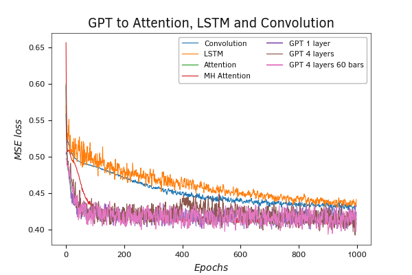
We performed the first test with all training parameters intact and a single layer in the GPT block. The graph of the model error in the learning dynamics has relatively large fluctuations. This can be caused by the unevenness of the data distribution between weight matrix updates due to a lack of data shuffling and a reduction in the amount of data fed into the model, which results in a decreased gradient error propagation to the weight matrix at each feed-forward iteration. I would like to remind you that during the implementation of the model, we discussed the issue of gradient error propagation only within the scope of the current state.
At the same time, despite the significant noise, the proposed architecture raises the quality bar for the model performance. It demonstrates the highest performance among all the models considered.
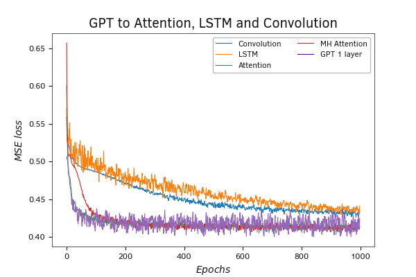
Testing the GPT model
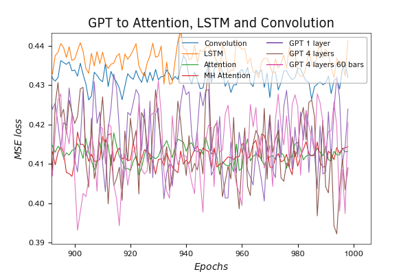
Zooming up the graph demonstrates how well the model lowers the minimum error threshold.
Here it should be added that during testing, we trained our model "from scratch". The authors of the architecture suggest unsupervised pre-training of the GPT block on a large dataset and then fine-tuning the pre-trained model for specific tasks during supervised learning.
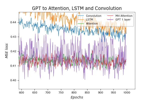
Testing the GPT model
Let's continue testing our implementation. All known implementations of the GPT architecture use multiple blocks of this architecture. For the next test, we increased the number of layers in the GPT block to four. The rest of the script parameters are left unchanged.
The testing results were as expected. Increasing the number of neural layers invariably leads to an increase in the total number of model parameters. A larger number of parameters requires a greater number of update iterations to achieve optimal results. In doing so, the model learns better to separate patterns and is more prone to overlearning. This is what the results of the model training demonstrated. We see the same noise in the error plot. In addition, we observe an even greater reduction in the minimum error metrics of the model.
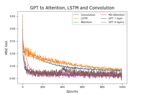
Testing the GPT 4 layer model
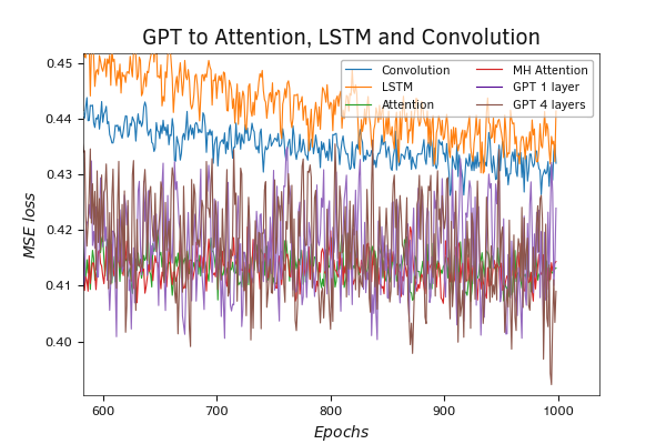
Testing the GPT 4 layer model
We would like to add that, from the practice of using attention models, their benefits are most clearly demonstrated when long sequences are used. GPT is no exception. It's more like the other way around. Since the model recalculates only the current state and uses archived copies of previous states, this significantly reduces the number of operations when analyzing large sequences. As the number of iterations decreases, the speed of the whole model increases.
For the next test, we increase the stack size to 60 candles. Thanks to the architectural design of GPT, we can increase the length of the analyzed sequence by simply increasing one external parameter without changing the program code. Among other things, we do not need to change the amount of data fed to the model input. It should be noted that changing the stack size does not change the number of model parameters. Yes, increasing the stack of Key and Value tensors leads to an increase in the Score vector of dependency coefficients. But there is absolutely no change in any of the weight matrices of the internal neural layers.
The test results demonstrated a reduction in the model's performance error. Moreover, the overall trend suggests that there is a high likelihood of seeing improved results from the model as we continue with further training.
Testing the GPT model with an enlarged stack
Testing the GPT model with an enlarged stack
We have constructed yet another architectural model of a neural layer. The testing results of the model using this new architectural solution demonstrate significant potential in its utilization. At the same time, we employed small models with rather short training periods. This is sufficient for demonstrating the functionality of architectural solutions but not adequate for real-world data usage. As practice shows, achieving optimal results requires various experiments and unconventional approaches. In most cases, the best results are achieved through a blend of different architectural solutions.