- Problem statement
- File arrangement structure
- Choosing the input data
- Creating the framework for the future MQL5 program
- Description of a Python script structure
- Fully connected neural layer
- Organizing parallel computing using OpenCL
- Implementing the perceptron model in Python
- Creating training and testing samples
- Gradient distribution verification
- Comparative testing of implementations
Comparative testing of implementations
In the previous section, we verified the correctness of the backpropagation algorithm operation. Now we can safely move on to training our perceptron. We will perform this work in the script perceptron_test.mq5. The first block of the script will remind you of the script from the previous section. This is a consequence of using our library to create neural networks. We will create a neural network using it. Hence, the algorithm for initializing and using the neural network will be identical in all cases.
To enable various testing scenarios, we will add the following external parameters to the script:
- The name of the file containing the training sample.
- The name of the file to record the dynamics of the error change. Using these values, we will be able to plot the error change graph during the training process, which will help us visualize the neural network learning process.
- The number of historical bars used in the description of one pattern.
- The number of input layer neurons per bar.
- Switch flag for using OpenCL technology in the process of training a neural network.
- Batch size for one iteration of weight matrix update.
- Learning rate.
- The number of hidden layers.
- The number of neurons in a single hidden layer.
- The number of iterations of updating the weight matrix.
Just like in the previous section, after declaring the external parameters in the global scope of the script, we will include our library for creating a neural network and declare an object of the base class CNet.
//+------------------------------------------------------------------+
|
Before moving on to writing the script code, let's consider what functionality we need to incorporate into it.
First, we need to create the model. For this, we will define the model architecture and call the model initialization method. Similar operations were performed in the script to check the correctness of the error gradient distribution.
Next, to train our model, we need to load the previously created training dataset, which will contain a set of input data and target values.
Only after successfully completing these steps, we can start the model training process. This is a cyclic process that includes a feed-forward pass, a backpropagation pass, and weight matrix updates. There are several approaches to the duration of model training. The most common one involves limiting the number of training epochs and tracking changes in the model error. We will use the first approach. The analysis of the error dynamics during the training process will allow us to develop criteria for applying the second method. Therefore, during training, we need to record the model error change and save the collected sequence after training. At the end of the training, we will save the obtained model.
Thus, we have defined the necessary functionality for our script. To create clear and readable code, we will divide it into blocks corresponding to the tasks mentioned above. In the body of the main function OnStart, we will sequentially call the corresponding functions with control over the execution of operations.
First, we will create a vector to record the dynamics of the model error during training. Its size will be equal to the number of training epochs.
//+------------------------------------------------------------------+
|
Next, we initialize our model for training. Here we instantiate a neural network class and pass the object pointer to the model initialization function. Be sure to check the result of the operation.
//--- 1. Initialize model
|
The next step is to load the training sample. For this purpose, we will need two dynamic arrays: one for loading the patterns of source data, and the other for the target values. Both arrays will be synchronized.
The data loading is performed in the LoadTrainingData function, in the parameters of which we will pass the file for data loading and pointers to the created dynamic array objects.
//--- 2. Load the training sample data
|
As mentioned earlier, after creating the model and loading the training dataset, we can start the training process. This functionality will be assigned to the NetworkFit method, in the parameters to which we will pass pointers to our model, a training sample with target values, and a vector recording the dynamics of the model error variation during training.
//--- 3. Train model
|
After completing the model training process, we save the history of the model error change during training. We will also keep the trained model. We do not need to create a separate function to save the trained model. We can use the previously created method of our base neural network class to save the model.
//--- 4. Save the error history of the model
|
To confirm the successful completion of all operations, we will print an informational message to the log and terminate the script.
As you can see, the code of the main function of the script turned out to be quite short, but clearly structured. This distinguishes it from the gradient distribution correctness check script in the previous section. The choice of programming style remains with the programmer and does not affect the functionality of our library. We go back to our script and now we will write the functions that we called above from the main function of the script.
First on the list is the NetworkInitialize model initialization function. In the parameters of this function, we pass a pointer to the object of the model being created. In the body of the function, we have to initialize the model before training. To initialize the model, we need to provide a description of the model to be created. I remind you that we create the model description in a dynamic array, each element of which contains a pointer to an instance of the object CLayerDescription with the description of the architecture of a specific neural layer. The very operation of creating such a model description has been moved to a separate function, CreateLayersDesc, which is a natural extension of the structured code concept.
//+------------------------------------------------------------------+
|
After creating the model architecture description, we call the initialization method of our neural network CNet::Create. Into it, we pass the description of the model architecture, the learning rate, optimization parameters, loss function, and regularization parameters. Don't forget to check the result of the model creation operations.
//--- initialize the network
PrintFormat("Error of init Net: %d", GetLastError());
|
After the successful initialization of the model, we set the flag for using OpenCL and set the batch size for model error averaging. In the provided example, regularization is set at the level of the weight matrix update batch.
To complete the description of the model initialization process, let's take a look at the CreateLayersDesc function, which is responsible for creating the architecture description of the model. In the parameters, the method receives a pointer to a dynamic array, into which we will write the architecture of the created model.
We first create a description of the initial data layer. The number of neurons in the input layer of the raw data depends on two external parameters: the number of historical bars in one pattern (BarsToLine) and the number of input layer neurons per bar (NeuronsToBar). The quantity is determined by their product. The input layer will be without an activation function and will not be trained. That's clear and should not raise any questions. In this layer, you're essentially storing the initial parameters from an external system in the results array of the layer. Within the layer, no operations are performed on the data.
bool CreateLayersDesc(CArrayObj &layers)
|
When using fully-connected neural layers, each neuron in the hidden layer can be considered as a specific pattern that the neural network learns during the training process. In this logic, the number of neurons in the hidden layer represents the number of patterns that the neural network is capable of memorizing. Certainly, you can establish a logical relationship between the number of elements in the previous layer and the number of possible combinations, which will represent patterns. But let's not forget that our previous neural layer results are non-binary quantities, and the range of variation is quite large. Therefore, the total number of possible combinatorial variants of patterns will turn out to be very large. The average probability of their occurrence will vary greatly. Indeed, most of the time, the number of neurons in each hidden layer will be determined by the neural network architect within a certain range, and the exact number is often fine-tuned based on the best performance on a validation dataset. For this reason, we gave the user the ability to specify the number of neurons in the hidden layer in the external parameter HiddenLayer. But let's say right away that we will create all neural layers of the same architecture and size.
The number of hidden layers depends on the complexity of the problem being solved and is also determined by the neural network architect. In this test, I will use a neural network with one hidden layer. However, I suggest that you independently conduct a few experiments with different numbers of layers and assess the impact of changing this parameter on the results. To perform such experiments, we have derived a separate external parameter — the number of HiddenLayers.
In practice, we create one hidden layer description and then add it to the dynamic array of architecture descriptions as many times as we need to create hidden neural layers.
//--- hidden layer
|
Within this section, I do not aim to fully train the neural network with the best possible results. We will only compare the performance of our library in different modes and their impact on learning outcomes. Let's also see in practice the impact of some of the approaches we discussed in the theoretical part of the book. Therefore, we will not delve deeply into the careful selection of architectural parameters for the neural network to achieve maximum results at this moment.
I have specified Swish as the activation function for the hidden layer. This is one of those functions whose range of values is limited at the bottom and not limited at the top. In this case, the function is differentiable over the whole range of permitted values. However, we will be able to evaluate other activation features during the testing process.
Choosing the activation function for the output layer is a compromise. The challenge here is that we have two goals: direction and strength of movement. This is not a standard approach to solving the problem, as our neural network output consists of two neurons with completely different values. One might consider the direction of movement as a binary classification (buy or sell), while determining the strength of movement is a regression task. It would probably be logical to train the neural network only to determine the strength of the movement, and the direction would correspond to the sign of the result. However, we are learning and experimenting. Let's observe the behavior of the neural network in such a non-standard situation. We will try to activate the neurons with a linear function, which is standard for solving regression tasks.
I have specified Adam as the training method for both neural layers.
The algorithm for describing neural layers is completely identical to the one discussed in the previous section. First, we describe each layer in an object of the CLayerDescription class. The sequence of describing layers corresponds to their sequence in the neural network, from the input layer of raw data to the output layer of results. As the layers are getting their descriptions, add them to the collection of the previously created dynamic array.
//--- results layer
|
The next step in our script was loading the training dataset in the LoadTrainingData function. We will load it from the file specified in the function parameters. In the body of the function, we immediately open the specified file for reading and check the result of the operation based on the value of the obtained handle.
//+------------------------------------------------------------------+
|
We will carry out the operation of loading the training sample in two steps. First, we will first patterns and target values into the two CBufferType buffers, piece by piece. We will collect the source data elements of one pattern in the pattern buffer and the relevant target results in the target buffer.
//--- display the progress of training data loading in the chart comment
|
After loading information about one pattern from the file, we will store pointers to objects with the data in two dynamic arrays, CArrayObj. We also got pointers to them in the function parameters. One array is used for source data patterns (data) and the second array is used for target values (targets). We repeat the operations in a loop until we reach the end of the file. To allow the user to monitor the process, we will display information about the number of loaded patterns on the chart in the comments field.
Note that since we are passing pointers to data objects into dynamic arrays, we need to create new instances of CBufferType objects after writing the pointers to the array. Otherwise, we will fill the entire dynamic array with a pointer to the same instance of an object, and the buffer will contain generic information about all patterns, the manipulation of which will require a different algorithm. Consequently, the entire neural network will not work correctly.
if(!data.Add(pattern))
|
After completing the loop for reading the data, we will obtain two arrays of objects with the same number of elements. In these, elements with the same index will constitute the source-target pair of the pattern data. Here we close the training sample file.
Now that we have the neural network already created and the training sample loaded, we can start training in the NetworkFit function. In its parameters, this method receives pointers to objects of the neural network and the training dataset. Additionally, it receives a pointer to a vector recording the dynamics of the model's error changes during the training process. To train the neural network, we will create two nested loops. We will initiate the first loop with the number of iterations equal to the external parameter Epochs which is the number of weight matrix updates. In the nested loop, we will create a number of iterations equal to BatchSize, i.e. the batch size to update the weights.
bool NetworkFit(CNet &net, const CArrayObj &data, |
In the body of the nested loop, we will randomly select one pattern from the training dataset. For each selected pattern, we will first make a forward pass on the corresponding input data. Then open the target values and do a backward pass.
//--- select a random pattern
|
By repeating iterations of feed-forward and backpropagation passes, we accumulate the error gradient on each element of the weight matrix. After completing the specified number of iterations of feed-forward and backpropagation passes up to the batch size for weight matrix updates, we exit the inner loop. Then we update the weights in the direction of the average gradient of the error, clear the buffer of accumulated error gradients, and save the current value of the loss function in a vector to monitor the training process. After that, we enter a new loop of training iterations.
//--- reconfigure the network weights
|
In the proposed example, the training process is constrained by an external parameter of the number of iterations of updating the weight matrix. In practice, a common approach is often used where the training process stops upon achieving specified performance metrics. This could be the value of the loss function, the accuracy rate of hitting expected results, and so on. A hybrid approach can also be employed, where both metrics are monitored while also setting a maximum number of training iterations.
After the training process is completed, we save the dynamics of the loss function to a file. This functionality is performed by the SaveLossHistory function, in the parameters of which we will pass the name of the file to record the data and the vector of dynamics of changes in the model error during training.
In the body of the function, we open or create a new CSV file to record the data and in a loop store all the model error values received during training.
void SaveLossHistory(string path, const VECTOR &loss_history)
|
After writing the data to the file, we close the file and output an informational message to the log indicating the full path of the saved file.
The presented example of the script implementation shows a full loading of the training sample into memory. Of course, working with RAM is always faster than accessing permanent memory. However, the sizes of the training dataset do not always allow it to be fully loaded into RAM. In such cases, the training sample is loaded and processed in batches.
Normalizing data at the neural network output
After creating such a script, we can conduct several instructive experiments. For example, we have previously discussed the importance of normalizing the initial data before feeding it to the input of a neural network. But how important is that? Why is it not possible to adjust the appropriate weights during the neural network training process to account for the data scale? Yes, we were talking about the impact of large values. But now we can do a practical experiment and see the effect of input data normalization on the model training result.
Let's take historical data for the EURUSD instrument, with a five-minute timeframe covering the period from 01.01.2015 to 12.31.2020, and create two training datasets: one with normalized data and the other with unnormalized data. Let's run the above neural network training script on both samples. We made the script for creating the training sample in Section 3.9.
The graph depicting the dynamics of the loss function says it all. The error on normalized data is much lower, even if we start with random weights. If the initial value of the loss function on unnormalized data is around 120, then on normalized data, it's only 0.6. Of course, during the training process, the value of the loss function on non-normalized data drops rapidly and after 200 iterations of weighting factor updates it drops to 6, and after 1000 iterations it reaches 4.5. But despite such a rapid rate of decline in the loss function index, it still significantly outperforms that for normalized data. On the final iterations, after 1000 weight matrix update iterations, the loss function approaches approximately 0.44.
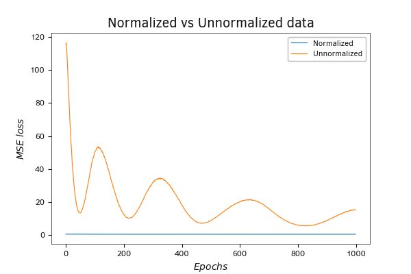
Graph of the dynamics of the MSE loss function during the training of a neural network, on both normalized and unnormalized data
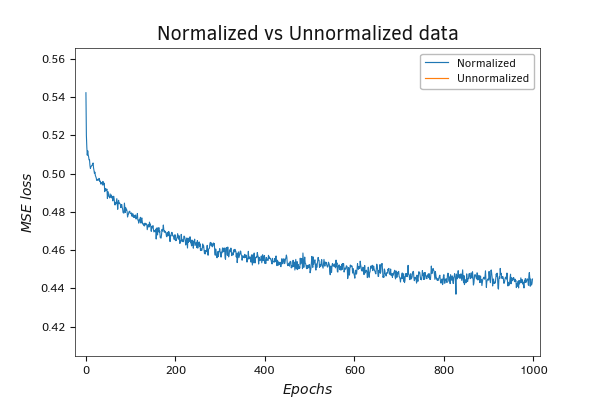
Graph of the dynamics of the MSE loss function during the training of a neural network, on both normalized and unnormalized data (scale)
I conducted a similar experiment both with and without using OpenCL technology. The results of the neural network were comparable. But in terms of performance on such a small neural network, the CPU won. Obviously, the data transfer overhead was much higher than the performance gains from utilizing multithreading technology. These results were expected. As we discussed earlier, using such technology is justified for large neural networks when the costs of data transmission between devices are offset by the performance gains achieved by splitting computational iterations into parallel threads.
I suggest repeating a similar experiment with your data — then you won't have any questions about the necessity of normalizing the input data. I believe that after conducting the experiment it is obvious that further testing should be performed on normalized data.
Choosing the learning rate
The next question that always arises for creators of neural networks is the choice of the learning rate. When tackling this issue, it's essential to strike a balance between performance and the quality of learning. Choosing an intentionally high learning rate allows for faster error reduction at the beginning of training. But then the rate of learning rapidly declines and at best stops far from the intended goal. In the worst case, the error starts to increase. Choosing an excessively small learning rate reduces the training speed. The process takes more time, and there's an increased risk of getting stuck in a local minimum without reaching the desired goal.
For experimental testing of the impact of learning rate on the neural network training process, let's train the previously created neural network using four different learning rates: 0.003, 0.0003, 0.00003 and 0.000003. The results of the test are shown in the graph below.
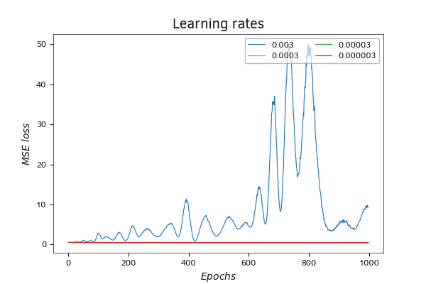
Comparison of the loss function dynamics when using different learning rates
During the training of the neural network using a learning rate of 0.003, fluctuations in the loss function are observed. During the learning process, the amplitude of the oscillations increases. In general, there is a tendency for the model error to increase. Such behavior is characteristic of an excessively high learning rate.
Reducing the learning rate makes the training schedule smoother. However, at the same time, the rate of decrease in the loss function value diminishes with each weight matrix update. The most gradual decrease in the loss function value is demonstrated by the training process with a learning rate of 0.000003. However, achieving the smoothness of the graph came at the cost of increasing the number of weight matrix update iterations required to reach the optimal result. Throughout the entire training process with 1000 weight matrix update iterations, a learning rate of 0.000003 exhibited the worst result among all.
Training the neural network with coefficients of 0.0003 and 0.00003 showed similar results. The loss function graph with a learning rate of 0.00003 turned out to be more jagged. But at the same time, the best result in terms of error value was shown by training with a rate of 0.0003.
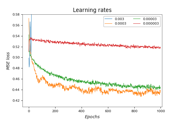
Comparison of the loss function dynamics when using different learning rates (scale)
Selecting the number of neurons in the hidden layer
The next aspect I'd like to demonstrate in practice is the impact of the number of neurons in the hidden layer on the training process and its outcome. When we talk about fully connected neural layers, where each neuron in the subsequent layer has connections to all neurons in the previous layer, and each connection is individual and independent, it's logical to assume that each neuron will be activated by its own combination of states from the neurons in the previous layer. Thus, each neuron responds to a different state pattern of the previous layer. Consequently, having a greater number of neurons in the hidden layer has the potential to memorize more such patterns and make them more detailed. At the same time, we are not programming pattern variations; we allow the neural network to learn them autonomously from the presented training dataset. It would seem that in this logic, increasing the number of neurons in the hidden layer can only increase the quality of training of the neural network.
But in practice, not all patterns have an equal probability of occurrence. The goal of training a neural network is not to memorize each individual state down to the finest details. Their goal is to use the training dataset to generalize the presented data, identify and highlight dependencies and regularities. The obtained data should allow the construction of a function that describes the relationship between the target values and the input data with the required accuracy. Therefore, an excessive increase in neurons in the hidden layer reduces the neural network's ability to generalize and leads to overfitting.
The other aspect of increasing the number of neurons in the hidden layer is the increase in the consumption of time and computational resources. The point is that adding one neuron in the hidden layer adds as many elements to the weight matrix as the previous layer contains plus one element for bias. Therefore, when choosing the number of neurons in the hidden layer, it's important to consider the balance between the achieved learning quality and the training costs for such a neural network. At the same time, you need to think about the risk of overfitting.
Certainly, there are established methods to combat overfitting in neural networks. These primarily include increasing the training dataset size and regularization techniques. We have discussed theoretical aspects of regularization earlier, and we will talk about practical applications a little later.
Now I suggest looking at the graphs of the error function values during the training of a neural network with a single hidden layer, where the number of neurons changes while keeping other conditions constant. When testing, I compared the training of 4 neural networks with 20, 40, 60 and 80 neurons in the hidden layer. Of course, such a number of neurons is too small to get any decent training results on a sample of 350 thousand patterns. Moreover, there is no risk of overtraining here. But they are enough to look at the impact of this factor on learning.
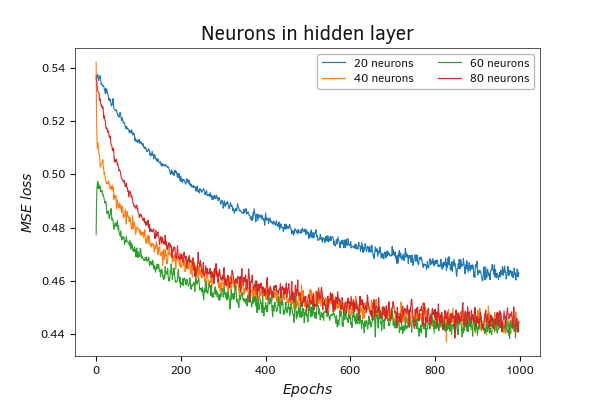
Comparison of the loss function dynamics when using different numbers of neurons in the hidden layer
As can be seen in the graph, the model with 20 neurons in the hidden layer showed the worst result. They are clearly insufficient for such a task.
Regarding the other three models, it can be said that the variation in the graphs during the first 100 weight update iterations can be attributed to the randomness factor due to initializing the models with random weights. After about 250-300 iterations of updates to the weight matrix, the graphs are intertwined into a single bundle and from this point go on together.
Increasing the scale of the graph allows us to identify the main trend: as the number of neurons in the layer increases, the number of iterations required to reach local minima and overall train the neural network also increases. At the same time, local minima of neural networks with a large number of neurons fall lower, and their graphs have a lower frequency of oscillations.
Overall, throughout the entire training process, the model with 60 neurons demonstrates the best performance. Slightly behind, almost in parallel, is the graph of the model with 40 neurons in the hidden layer. For a model with 80 neurons in the hidden layer, 1000 iterations of updating the weight matrix were insufficient. This model shows a slower decrease in the value of the loss function. At the same time, the dynamics of the loss function values graph demonstrate the potential for further reducing the loss function value with continued training of the model. There are valid reasons to expect a decrease in the performance achieved by the model with 60 neurons in the hidden layer.
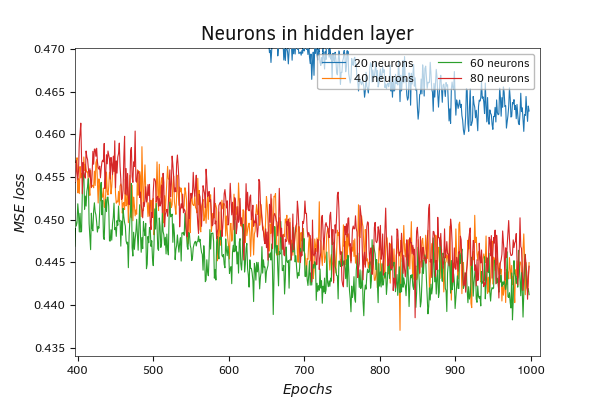
Comparison of loss function dynamics using different numbers of neurons in the hidden layer (scale)
However, it's important to note that a decrease in error on the training dataset could also be associated with model overfitting. Therefore, before the practical deployment of a trained model, it's always important to test it on "unseen" data.
Training, validation, testing.
During training, we adjust the weight matrix parameters to achieve the minimum error on the training dataset. But how will the model behave on new data beyond the training sample? It's also important to consider that we are dealing with non-static data that is constantly changing, influenced by a large number of factors. Some of these factors are known to us, while we might not even be aware of others. And even about the factors known to us, we cannot say with certainty how they will change in the future. Moreover, we don't know how this will impact the variation of the data we are studying. It is most likely that the performance of the neural network will deteriorate on the new data. But what will that deterioration be? Are we willing to accept such risks?
The first step towards addressing this issue is the validation of the model's training parameters. For model validation, a dataset that is not part of the training set is used. Most often, the entire set of initial data is divided into three blocks:
- training sample (~60%)
- validation sample (~20%)
- test sample (~20%)
The percentage distribution for each dataset is given as an example and can vary significantly depending on the specific task at hand.
The essence of the validation process lies in testing the parameters of the trained model on data that is not part of the training dataset. During validation, hyperparameters of the trained model are tuned to achieve the best possible performance.
When writing a script for a fully connected perceptron in Python, we allocated 20% of the training dataset for validation. The training of the first model demonstrated results similar to those obtained when training the model created in MQL5. That's a positive signal for us. Obtaining similar results when training models created in three different programming languages can indicate the correctness of the algorithm we have implemented.
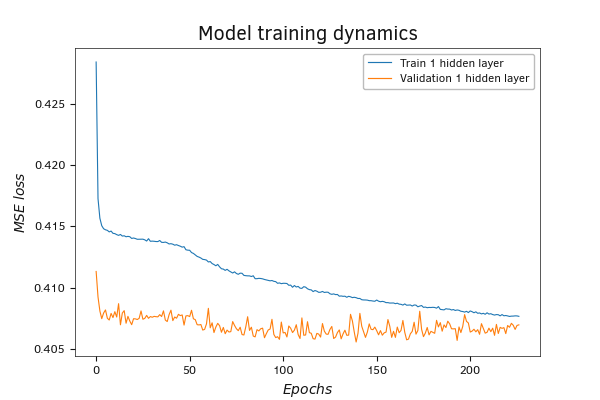
Change in performance of a model with a single hidden layer on validation at pace with its training
Evaluating the graphs of the test results, one can notice a tendency for the error to decrease during the learning process. This is a positive signal that indicates the model's ability to learn and establish relationships between input data and target labels. At the same time, there's an increase in error on the validation data, which could indicate both the overfitting of the model and the non-representativeness of the validation dataset.
The issue might be that we specified a portion of the data for validation within the training dataset. In this case, the TenzorFlow library takes the latest data in the training sample set. However, this approach doesn't always yield accurate results, as the outcomes of individual periods can be significantly influenced by local trends.
In the graph below, I can see the impact of both factors. The overall trend of increasing error on the validation data indicates the model's tendency to overfit, while the initial validation error being lower than the training error might be due to the influence of local trends.
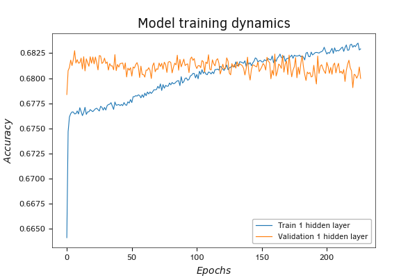
Change in performance of a model with a single hidden layer on validation at pace with its training
The graph of the accuracy metric shows similar trends. The metric itself reflects the model accuracy as a proportion of correct answers in the total number of results. Here we observe an increase in the indicator during training with an almost unchanged indicator on validation. This may indicate that the model learns patterns that do not occur in the validation sample.
In theory, adding hidden layers should enhance the model's ability to learn and recognize more complex patterns and structures. We created the second model in Python with three hidden layers. Indeed, in this model in training, the error decreased significantly. But at the same time, it has further increased in the validation process. This is a clear sign of the model overfitting. When the model, due to its capabilities, does not generalize dependencies and simply "memorizes" pairs "initial data - target values", the result appears randomly on new data not included in the training sample.
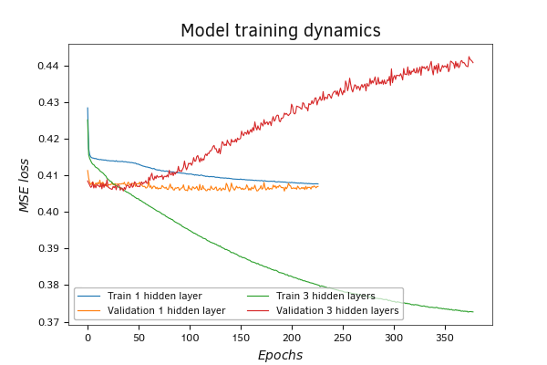
Change in performance of a model with three hidden layers on validation at pace with its training
The dynamics of the accuracy metric have trends similar to those of the loss function. The only difference is that the loss function decreases during the training process, while the accuracy increases.
One way to combat overfitting is to regularize the model. We added ElasticNet regularization to the third model, and it did the job. When the model was trained with regularization, the error decreased at a slower rate. At the same time, the increase in error on the validation set has slowed down.
Once again, on the accuracy metric graph, we observe the same trends as on the loss function graph.
Note that the training and regularization parameters were not meticulously tuned. Therefore, learning outcomes cannot be considered definitive.
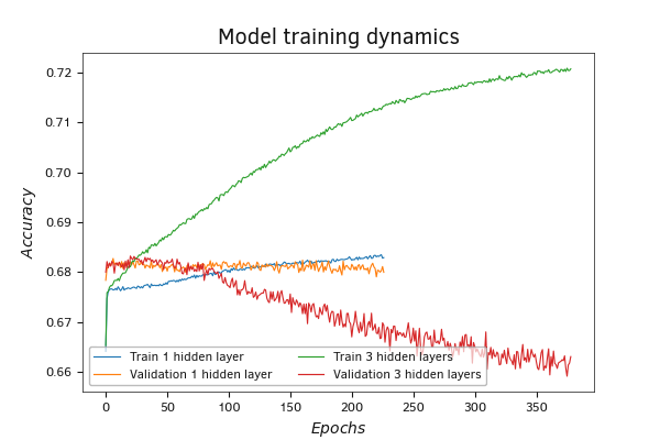
Change in performance of a model with three hidden layers on validation at pace with its training
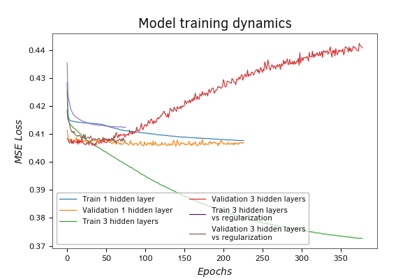
The change in the performance of the model with three hidden layers and regularization on validation is occurring at a similar pace to its training.
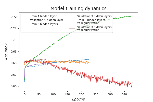
The change in the performance of the model with three hidden layers and regularization on validation is occurring at a similar pace to its training.
After training the models, we will evaluate them using the test dataset. In contrast to validation, the model with three hidden layers and no regularization demonstrated the lowest error on the test dataset. The model with regularization showed the maximum error. Such differences in results between the test and validation datasets can possibly be explained by the way the datasets were created. While the validation sample included only the most recent data from the training sample, the test sample collected random data sets from the entire population. Thus, the test sample can be considered more representative, as it is deprived of the influence of local tendencies.
Measuring the accuracy metric on the test sample showed similar results. The best result was obtained on the model with three hidden layers.
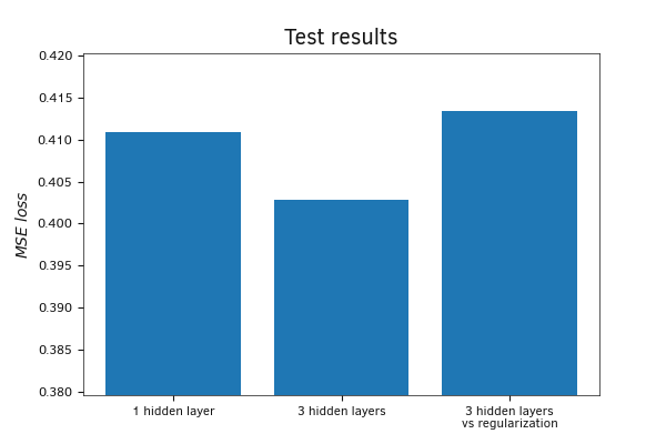
Comparison of model results on a test sample
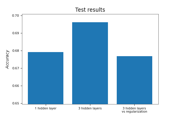
Comparison of model results on a test sample
We can summarize the results of our practical work.
- Normalizing the raw data before feeding it to the input of the neural network greatly increases the chances of convergence of the neural network and reduces the training time.
- The learning rate should be carefully selected experimentally. Too high learning rates lead to unbalancing of the neural network and an increase in error. Too low learning rates lead to more time and computational resources spent on training the neural network. This increases the risk of stopping the learning process at a local minimum without achieving the desired result.
- Increasing the number of neurons in the hidden layer gives improved results of training. But at the same time, training costs are also rising. When choosing the size of the hidden layer, it is necessary to find a balance between the training error and the resource cost of conducting the training of the neural network. It should be kept in mind that an excessive increase in the number of neurons in the hidden layer increases the risk of neural network overfitting.
- Increasing the number of hidden layers also increases the model's ability to learn and recognize more complex shapes and structures. In this case, the model's propensity to overfitting increases significantly.
- The use of a set of recent training sample values for validation is not always able to show true trends, as such a validation sample is strongly influenced by local trends and cannot be representative.
However, we are building a model for financial markets. It is important to us to make a profit both in the long term and in the present moment. Of course, there may be some localized losses, but they should not be large and frequent. Therefore, it is important to obtain acceptable results both on a single localized dataset and on a more representative sample. Probably, getting better results on a local segment has a higher impact: after making a local profit, we can retrain the model to adapt to new trends and make a profit on a new local segment. At the same time, if training costs exceed possible local losses, the profitability over a long period using a representative sample becomes more significant.