- Problem statement
- File arrangement structure
- Choosing the input data
- Creating the framework for the future MQL5 program
- Description of a Python script structure
- Fully connected neural layer
- Organizing parallel computing using OpenCL
- Implementing the perceptron model in Python
- Creating training and testing samples
- Gradient distribution verification
- Comparative testing of implementations
Choosing the input data
Having defined the problem statement, let's now turn our attention to the selection of input data. There are specific approaches to this task. At first glance, it might seem like you could load all available information into the neural network and let it learn the correct dependencies during training. This approach will prolong learning indefinitely, without guaranteeing the desired outcome.
The first challenge we face is the volume of information. To convey a large amount of information to the neural network, we would need a considerably large input layer of neurons with a substantial number of connections. Hence, more training time will be required.
Furthermore, we will encounter the issue of data incomparability. Samples of different metrics will have very different statistical characteristics. For example, the price of an instrument will always be positive, while its change can be both positive and negative.
Some indicators have normalized values and others do not. The magnitudes of values for various indicators and the amplitude of their changes can differ by orders of magnitude. However, their impact on the outcome may be comparable, or an indicator with lower values may have an even greater impact.
Such a situation will significantly complicate the training process, as it will be challenging to discern the impact of small values within an array of large values.
Another problem lies in the use of highly correlated features. The presence of a correlation between features can indicate either a cause-and-effect relationship between them or that both variables are dependent on a common underlying factor. Consequently, the use of correlated variables combines the two mentioned problems and their consequences. Using multiple variables depending on one factor exaggerates its impact on the overall outcome. Unnecessary neural connections complicate the model and delay learning.
Selecting features
Let's undertake preparatory work, taking into account the considerations mentioned above. Of course, we won't manually select and compare data, as we live in the era of computer technology. To calculate the correlation coefficient, let's create a small script in the file initial_data.mq5.
As a reminder, according to the previously described directory structure, all scripts are saved in the folder terminal_dir\MQL5\Scripts. For the scripts in our book, we will create the NeuroNetworksBook subdirectory, and for all the scripts in this chapter, we will create the initial_data subdirectory. So the full path of the file to be created will be:
- terminal_dir\MQL5\Scripts\NeuroNetworksBook\initial_data\initial_data.mq5
We will directly calculate the correlation coefficient using the Mathematical Statistics Library from the MetaTrader 5 platform. In the script header, include the necessary library, and in the external parameters, specify the period for analysis.
#include <Math\Stat\Math.mqh> |
When you run a script, MetaTrader 5 generates a Start event that is handled by the OnStart function in the script body. At the beginning of this function, we get multiple indicator handles for further analysis.
Note that first on my list of indicators is ZigZag, which we will use to get reference values when training the neural network. Here, we will use it to check the correlation of indicator readings with reference values.
Indicator settings are defined by the user at the problem statement stage. The neural network will be trained on the M5 timeframe data, so I set the Depth parameter to 48, which corresponds to four hours. In this way, I expect that the indicator will reflect 4-hour extremes.
The selection of the indicators list and parameters is up to the neural network architect. Parameter tuning is also possible when assessing correlation, which we will explore a bit later. At this stage, let us specify the indicators and their parameters from our subjective considerations.
void OnStart(void) |
The next step is to load historical quotes and indicator data. To obtain historical data, we will create a series of arrays with names corresponding to the names of indicators and quotes. This will help us avoid confusion while working with them.
Price data in MQL5 can be obtained by CopyOpen, CopyHigh, CopyLow, and CopyClose functions. The functions are created according to the same template, and it is clear from the function name which quotes it returns. The CopyBuffer function is responsible for receiving data from indicator buffers. The function call is similar to the function for obtaining quotes, with the only difference being that the instrument's name and timeframe are replaced with the indicator handle and the buffer number. I'll remind you that we obtained the indicator handles a little earlier.
double close[], open[],high[],low[]; |
All functions write data to the specified array and return the number of copied values. So, when making the call, we check for the presence of loaded data, and if there is no data, we exit the script. In this case, we'll give the terminal some time to load quotes from the server and recalculate indicator values. After that, we will rerun the script.
double zz[], cci[], macd_main[], macd_signal[],rsi[],atr[], bands_medium[]; |
As mentioned above, not all variables are comparable. Although linear transformations will not significantly affect the correlation coefficient, we still need to preprocess some values.
First, this applies to parameters that directly point to the instrument price. Since our goal is to create a tool capable of projecting accumulated knowledge onto future market situations, where there will be similar price movements but at a new price level, we need to move away from absolute price values and move toward a relative range.
So, instead of using the candlestick opening and closing prices, we can take their difference (the size of the candlestick body) as an indicator of price movement intensity. We will also replace the High and Low candlestick extremes with their deviation from the opening or closing price. We will treat SAR and Bollinger Bands indicators in the same way.
Remember the classic MACD trading rules. In addition to the actual indicator values, their position relative to the signal line within the histogram is also crucial. To test this relationship, lets add the difference between the indicator lines as another variable.
Now, let's address our reference point for the price movement. The ZigZag indicator gives absolute price values of extremes on a particular candlestick. However, we ideally want to know the price reference point for each market situation. In other words, we need a price guide for the upcoming movement on each candlestick. In doing so, we will consider two options for such a benchmark:
- Direction of movement (vector target1).
- Magnitude of movement (vector target2).
We can solve this task using a loop. We will iterate over the ZigZag indicator values in reverse order (from the newest values to the oldest values). If the indicator finds an extremum, we will save its value in a local variable extremum. If there is no extremum, we will use the last saved value.
Simultaneously, in the same loop, we will calculate and save the target values for our dataset. For this, we will subtract the closing price of the analyzed bar from the price value of the last peak. This way we get the magnitude of the movement to the nearest future extremum (target2 vector). The sign of this value will indicate the direction of movement (vector target1).
int total = ArraySize(close); |
double extremum = -1; |
After completing the preparatory work, we will proceed to check the data correlation. Since we'll be performing the same operation for different indicator data, it makes sense to encapsulate this iteration in a separate function. From the body of the Start function, we will only make the function call, passing different source data to it. The results of the correlation analysis will be saved to a CSV file for further processing.
int handle = FileOpen("correlation.csv", FILE_WRITE | FILE_CSV | FILE_ANSI,
|
Correlation(target1, target2, bands_medium, "BB Main", handle); |
The algorithm of our correlation test method is pretty straightforward. The correlation coefficient is calculated using the MathCorrelationPearson function from the MQL5 standard statistical analysis library. We will call this function sequentially for two sets of data:
- Indicator and direction of the upcoming movement; and
- Indicator and strength of the upcoming movement.
The results of the analysis are used to form a text message, which is then written to a local file.
void Correlation(double &target1[], double &target2[], |
The results of my analysis are presented in the graph below. The data show that there is no correlation between our target data and the ATR indicator values. The deviation from the extremes of the candlestick to its closing price (High — Close, Close — Low) also shows a low correlation with the expected price movement. Consequently, we can safely exclude these figures from our further analysis.
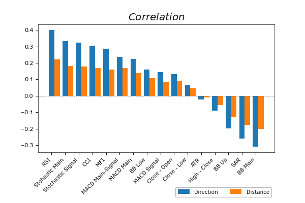
Correlation of indicator values with expected price movements
In general, the conducted analysis shows that determining the direction of the upcoming movement is much easier than predicting its strength. All indicators showed a higher correlation with the direction rather than the magnitude of the upcoming movement. However, the correlation with all values remains rather low. The RSI indicator demonstrated the highest correlation, with a value of 0.40 for the direction and 0.22 for the magnitude of the movement.
The correlation coefficient takes values from -1 (inverse relationship) to 1 (direct relationship), with 0 indicating a complete absence of dependence between random variables.
It's worth noting that among the three arrays of data obtained from the MACD indicator (histogram, signal line, and the difference between them), it's the distance between the MACD lines that demonstrated the highest correlation with the target data. This only confirms the validity of the classical approach to using indicator signals.
The next step is to test the correlation between data from different indicators. To avoid comparing each indicator with all others, we will analyze the correlation of indicators with RSI (the winner of the previous stage). We will perform the task using the previously created script with minor modifications. The new script will be saved in the file initial_data_rsi.mq5 in our subdirectory.
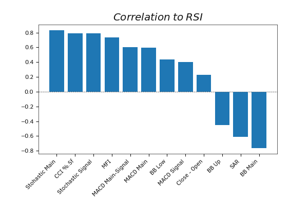
Correlation of indicator values to RSI
The analysis showed a strong correlation of RSI with a range of indicators. Stochastic, CCI, and MFI have a correlation coefficient with RSI which is greater than 0.70, while the main line of Bollinger Bands showed an inverse correlation of -0.76 with RSI. This indicates that the indicators mentioned above will only duplicate signals. Including them for analysis in our neural network will only complicate its architecture and maintenance. The expected impact of their use will be minimal. Therefore, we are excluding the aforementioned indicators from further analysis.
The indicators that show the minimum correlation with RSI are the two deviation variables:
- MACD signal line (0.40);
- Between opening and closing prices (0.23).
The deviation of the MACD signal line from the histogram in the first step showed a strong correlation with the target data of the upcoming price movement. Based on this data, it is MACD that will be taken into our indicator basket. Next, we will check its correlation with the remaining indicators.
The updated script is saved in the file initial_data_macd.mq5 in the subdirectory.
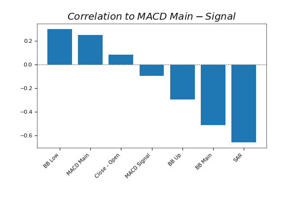
Correlation of indicator values to MACD Main-Signal
The SAR indicator here shows some interesting data. With moderate levels of inverse correlation to the target data, it shows a relatively high negative correlation with both selected indicators. The correlation coefficient with MACD was -0.66 and for RSI it was -0.62. This gives us reason to exclude the SAR indicator from the basket of analyzed indicators.
A similar situation is observed for all three Bollinger Bands indicator lines.
So far, we have selected two indicators for our indicator basket for further training of the neural network.
But this is not the end of the road to initial data selection. It should be noted that the neural network analyzes linear dependencies between the target values and the initial data in their pure form. So, it analyzes the data that is input into it. Each indicator is analyzed in isolation from other data available on the neuron input layer.
Hence, the neural network won't be able to capture the relationship between the source data and target values if it's not a linear relationship, such as being power law or logarithmic instead. To find such relationships, we need to prepare data beforehand. And to test the usefulness of such work, we need to test the correlation between such values.
In the script initial_data_rsi_pow.mq5, we will analyze the change in correlation with the expected price movement when the RSI indicator values are set to different degrees. The new script can be saved in the appropriate subdirectory.
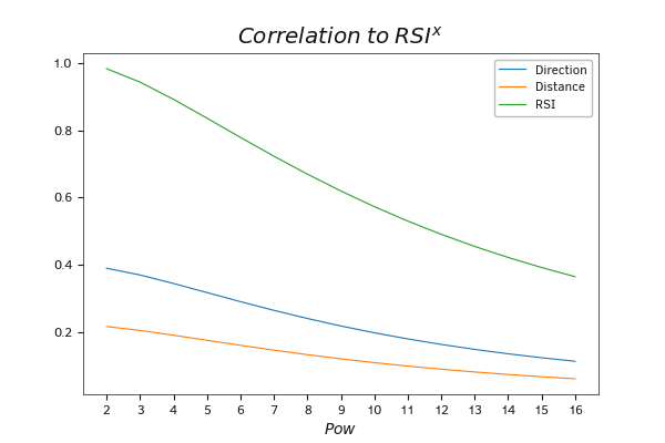
The dynamics of how the correlation of RSI values changes in relation to the expected movement when raising the indicator to a power.
The presented graph clearly shows that as the exponentiation of the indicator values increases, the correlation with the original values decreases much faster than with the expected price movement. This observation gives us a potential opportunity to expand the basket of original data indicators with exponential values of the selected indicators. A little later, we will be able to see how it works in practice.
It's important to note that when using exponential operations on indicators, you need to consider the properties of exponents and the nature of indicator values. Indeed, when raising any number to an even exponent, the result will always be positive. In other words, we lose the sign of the number.
For example, if we have two equal-magnitude values of a certain indicator with opposite signs, and they correlate with the target data. If the indicator is positive, the target function grows and if it is negative, it falls. Squared values for such an indicator will give us the same value. In this case, we will observe a decrease in correlation or a complete absence of it, as our target function remains unchanged while the indicator loses its sign.
This effect is noticeable when analyzing the change in correlation when raising the power of the difference between the lines of the MACD indicator, which we conducted in the script initial_data_macd_pow.mq5 from our subdirectory.
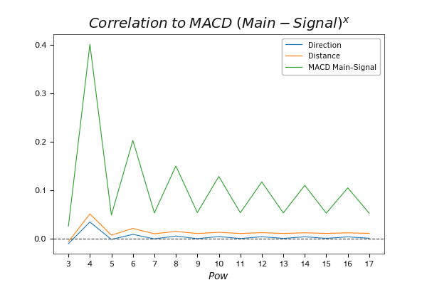
Dynamics of changing the correlation of MACD values to expected movement when raising the indicator to the power
Similarly, you can test the correlation of various indicators with the target values. The only limit is your ability and common sense. In addition to standard indicators and price quotes, these could also include custom indicators, and quotes from other instruments, including synthetic ones. Don't be afraid to experiment. Sometimes you can find good indicators in the most unexpected places.
Effect of the time shift on the correlation coefficient
After selecting the indicators for analysis, let's remember that we are dealing with time series data. One of the features of time series is their "historical memory". Each subsequent value depends not only on one previous value but also on a certain depth of historical values.
Certainly, one approach could be experimental — building a neural network and conducting a series of experiments to identify the optimal configuration. In this approach, it will take time to create and train several experimental models. Optionally, we could use our sample to test the correlation of the data with the historical shift.
To solve this problem, let's modify the script slightly and replace the Correlation function with ShiftCorrelation. The new function is a complete descendant of the Correlation function and is built using the same algorithm.
In the function parameters, we add a new variable max_shift to which we pass the maximum shift for analysis.
Time offsets are organized by copying the data to the new shifted arrays. The initial data will be copied without offset but to a lesser extent. Data reduction corresponds to time offset. At the same time, we will transfer the target values data to new arrays with offsets. However, since the size of the target data in our dataset is constant, when shifting, the number of elements for correlation analysis decreases. Therefore, after copying the data, we get data sets that are comparable in size and with a given time shift.
All we need to do is call the correlation coefficient calculation function and write the resulting data to a file.
To analyze the change in correlation with the increase in displacement over time, wrap all operations in a loop. The number of looping iterations corresponds to the max_shift parameter.
void ShiftCorrelation(double &targ1[], double &targ2[], |
string message; |
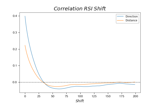
Dynamics of the correlation between RSI values and the expected movement, with time shift
To analyze the effect of shifting RSI indicator values over time on the correlation with target data, we will create a new script in the file initial_data_rsi_shift.mq5 in the specified initial_data_rsi_shift.mq5 subdirectory.
The results of the analysis show a rapid decline in the correlation up to the 30th bar. Then, a slight inverse correlation with a peak coefficient of -0.042 is observed around the 60th bar, followed by a gradual approach to 0. In such a situation, the use of the first 30 bars would be most effective. Further expansion of the analysis depth may lead to a decrease in the efficiency of utilizing computational resources. The value of such a solution can be tested in practice.
A similar analysis of MACD indicator data in the script initial_data_macd_shift.mq5 showed a similar dynamic with a slight shift in the transition zone from direct to inverse correlation at around the 40th bar.
Thus, conducting a correlation analysis of available source data and target values allows us to choose the optimal set of indicators and historical depth during the preparatory phase. This helps in analyzing data and forecasting target values more effectively. This enables us to significantly reduce expenses during the neural network creation and training phases with relatively low effort spent on the preparatory stage.
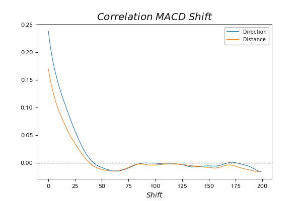
Dynamics of the correlation between MACD values and the expected movement, with time shift